options(rmarkdown.html_vignette.check_title = FALSE)
# Package imports
library(ape)
library(DECIPHER)

# Helper plotting function
plot_tree_unrooted <- function(dend, title){
  tf <- tempfile()
  WriteDendrogram(dend, file=tf, quoteLabels=FALSE)
  predTree <- read.tree(tf)
  plot(predTree, 'unrooted', main=title)
}
Distance Matrices
Most phylogenetic reconstruction algorithms rely upon constructing distance matrices. There are a variety of way to do this, but for purposes of illustration we’ll just be using Hamming Distance, which is one of the simplest methods. More complex methods can use nucleotide or amino acid substitution models.
Let’s construct a toy dataset for purposes of illustration:
sequenceSet <- DNAStringSet(c('AGACT',
                              'AGACG',
                              'TCATT',
                              'TGCTG',
                              'AGCTG'))
names(sequenceSet) <- 1:5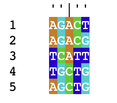
For each pair of sequences, we count the proportion of residues that do not match and mark this as the distance between them. As an example of calculating distance, consider the first two sequences in this set:
\[\begin{align*} &1)\;\;&AGACT&\\ &2)\;\;&AGACG& \end{align*}\]
Since these sequences differ at 1 out of 5 total residues, their distance is \(\frac{1}{5}=0.2\).
We can quickly calculate a complete distance matrix between these sequences with the following:
dm <- DistanceMatrix(sequenceSet, type='dist', verbose=F)
dm
## 1 2 3 4 5
## 1 0.0 0.2 0.6 0.8 0.6
## 2 0.2 0.0 0.8 0.6 0.4
## 3 0.6 0.8 0.0 0.6 0.8
## 4 0.8 0.6 0.6 0.0 0.2
## 5 0.6 0.4 0.8 0.2 0.0Notice that the distance between 1 and 2 is 0.2, just as we calculated before. Now we can begin to create trees.
Ultrametric Trees
UPGMA
The simplest tree building method is the Unweighted Pair Group Method with Arithmetic Means (UPGMA). This is a hierarchical clustering algorithm that sequentially builds a tree from the bottom up. The algorithm begins with a distance matrix, and proceeds in the following steps:
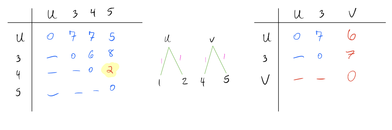
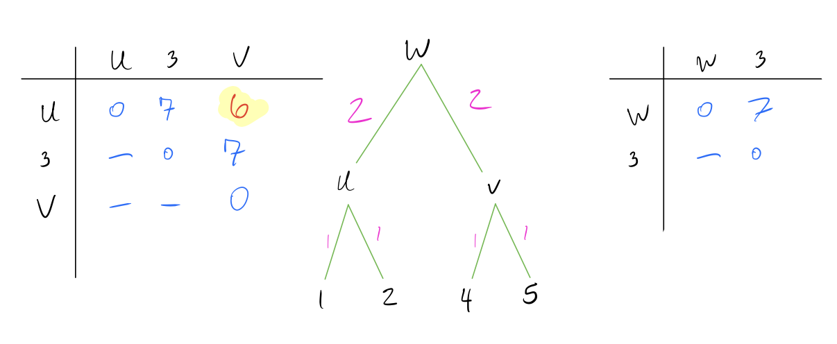
Identify the pair of nodes with the lowest distance \(d_{min}\). Here I’ve multiplied the distances by 10 to make it easier to read (it doesn’t make a difference in the final result).
Create a new node \(N_{new}\) that joins these pairs of nodes, and create branch lengths such that each leaf is equidistant from \(N_{new}\) The total branch length should from the \(N_{new}\) to any leaf should be half of \(d_{min}\). In this case, \(d_{min} = 2\) and our new node is called \(u\).
Combine the two rows of the distance matrix into one row by replacing each pair of entries with their average. The average is weighted by the number of leaves in each pair being combined, so if the two rows are each clusters with multiple leaves, the average should be weighted accordingly.
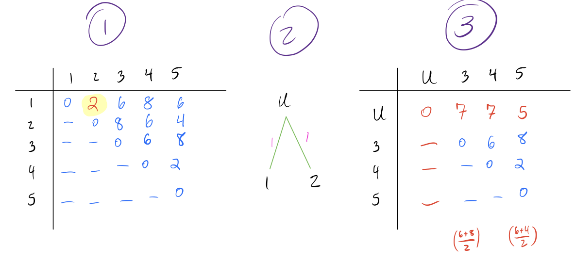
- Repeat above steps until all nodes are combined and the distance matrix is a single row and column.
Note that UPGMA methods always create an ultrametric tree, which means the tree is rooted and all leaves are equidistant from the root. This implies a molecular clock (rate of mutation is the same across all lineages of a tree).
WPGMA
A variation of UPGMA is WPGMA, where W stands for ‘weighted’. The difference between UPGMA and WPGMA is a bit counter-intuitive. Recall that when we combine two rows of the distance matrix in UPGMA, we weight our average by the number of leaves in the node being combined. In WPGMA, we do not weight by number of leaves in the node, and instead treat each node as having equal weight.
As an example, consider the following distance matrix:
\[ \begin{matrix} & n_1 & n_2 & n_3 \\ n_1 & 0 & 3 & 5 \\ n_2 & - & 0 & 3 \\ n_3 & - & - & 0 \\ \end{matrix}\]
Now suppose that node \(n_1\) has 10 leaves, node \(n_2\) has 2 leaves, and node \(n_3\) has 1 leaf. If we wanted to combine nodes \(n_1\) and \(n_2\) into node \(u\) using UPGMA, the distance from \(u\) to \(n_3\) would be calculated with the following formula:
\[\begin{align*} d_{UPGMA}(u, n_3) &= \frac{1}{|n_1| + |n_2|} \left(|n_1|*d(n_1,n_3) + |n_2|*d(n_2,n_3) \right)\\ \\ &= \frac{1}{10+2} \left(10*5 + 2*3 \right) \\ \\ &= 4.67 \end{align*}\]
However, if we combined these with WPGMA, we would instead ignore the number of leaves in each cluster and just take the simple arithmetic average, as follows:
\[\begin{align*} d_{WPGMA}(u, n_3) &= \frac{1}{2} \left(d(n_1,n_3) + d(n_2,n_3) \right)\\ \\ &= \frac{1}{2} \left(5 + 3 \right) \\ \\ &= 4 \end{align*}\]
You’re probably wondering, “why does weighted PGMA use unweighted combinations and vice-versa?” The answer lies in what we’re referring to when we talk about pair combinations being (un)weighted. Since UPGMA weights each node by the number of leaves, it’s correcting for nodes representing clades of difference sizes. In other words, the combination is inherently weighted, and UPGMA uses a clever way to “undo” this combination. WPGMA, by contrast, does not weight by clade size, and thus the combinations are biased (weighted) by the number of leaves in each nodes.
R Implementation
We can create a UPGMA tree in R with the below commands. Note that R doubles the lengths obtained by this, so I’m going to multiply the distance matrix by 5 to get the same scale factor as the example worked through above.
# UPGMA Tree
dend <- as.dendrogram(hclust(dm*5, method='average'))
plot(dend)
Implementing WPGMA trees is very similar to UPGMA trees (and gives the same result in this example):
# WPGMA Tree
dend <- as.dendrogram(hclust(dm*5, method='mcquitty'))
plot(dend)
There are also other methods for combining the distance matrices–see
the help page for hclust for other examples.
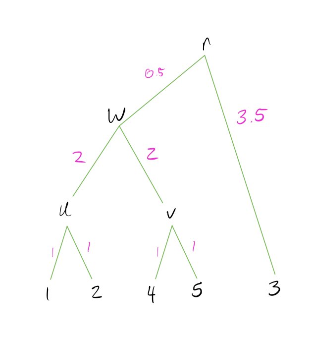
Neighbor Joining Trees
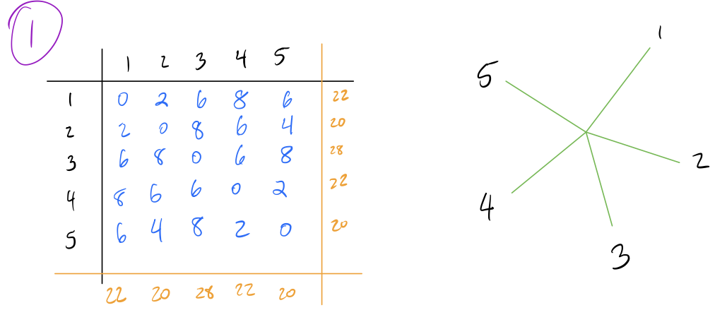
Another common approach to building trees is the Neighbor-Joining (NJ) method. This method also utilizes distance matrices, but proceeds from the top-down rather than UPGMA’s bottom-up approach. We’ll use the same distance matrix (multiplied by 10 as before for simpler visualization).
Algorithm
The algorithm proceeds in the following steps:
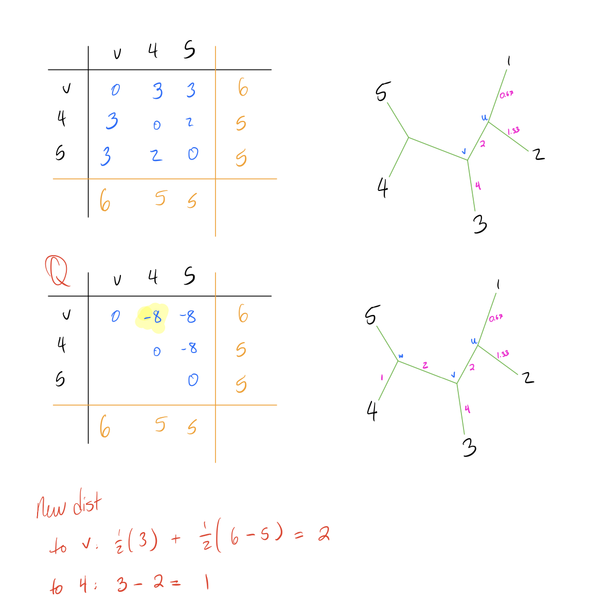
- Start with a star tree (all connected to a single root node), and record the row and column sums for each row/column of the matrix.
- Create a Q-matrix, which is a matrix of the same dimensions as the distance matrix, and each element given by the following formula:
\[Q[i,j] = (n-2)d(i,j) - R(i) - C(j)\]
rows of the distance matrix), \(d(i,j)\) is the distance from node \(i\)
to node \(j\), \(R(i)\) is the sum of the \(i\)’th row, and \(C(j)\) is the sum
of the \(j\)’th column.
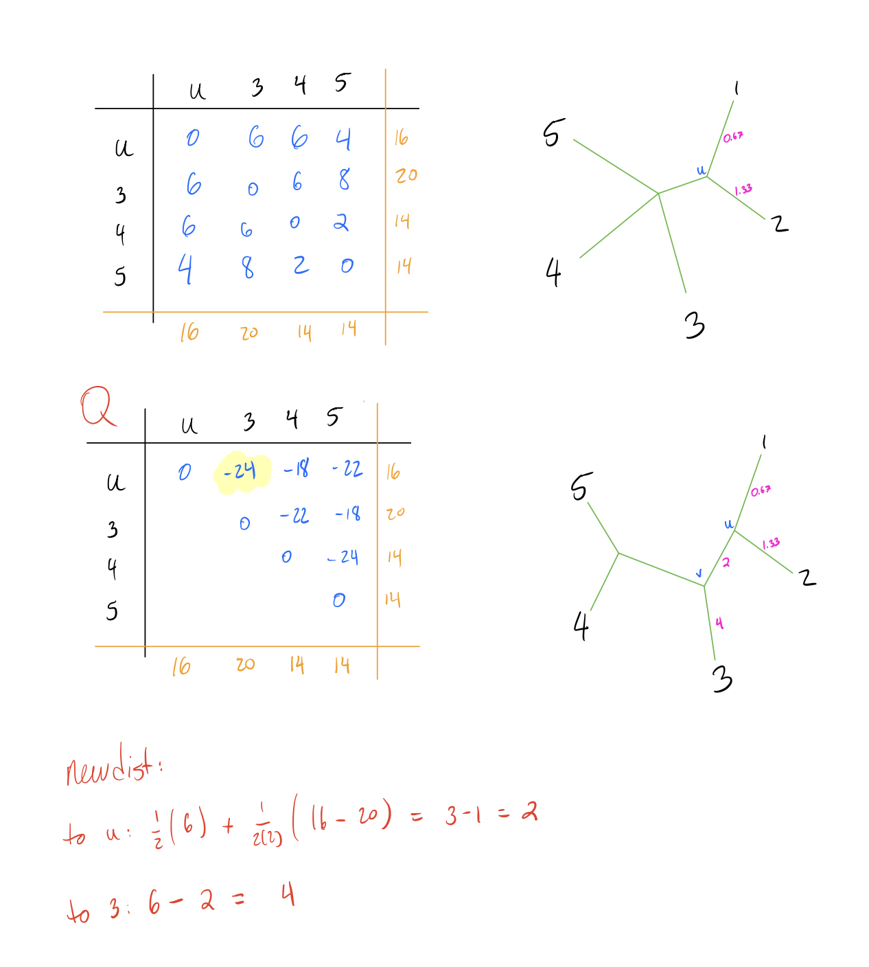
- Identify the smallest pair \(f,g\) in the Q-matrix, and combine the corresponding nodes by adding an intermediate node \(N_{int}\) between them in the tree.
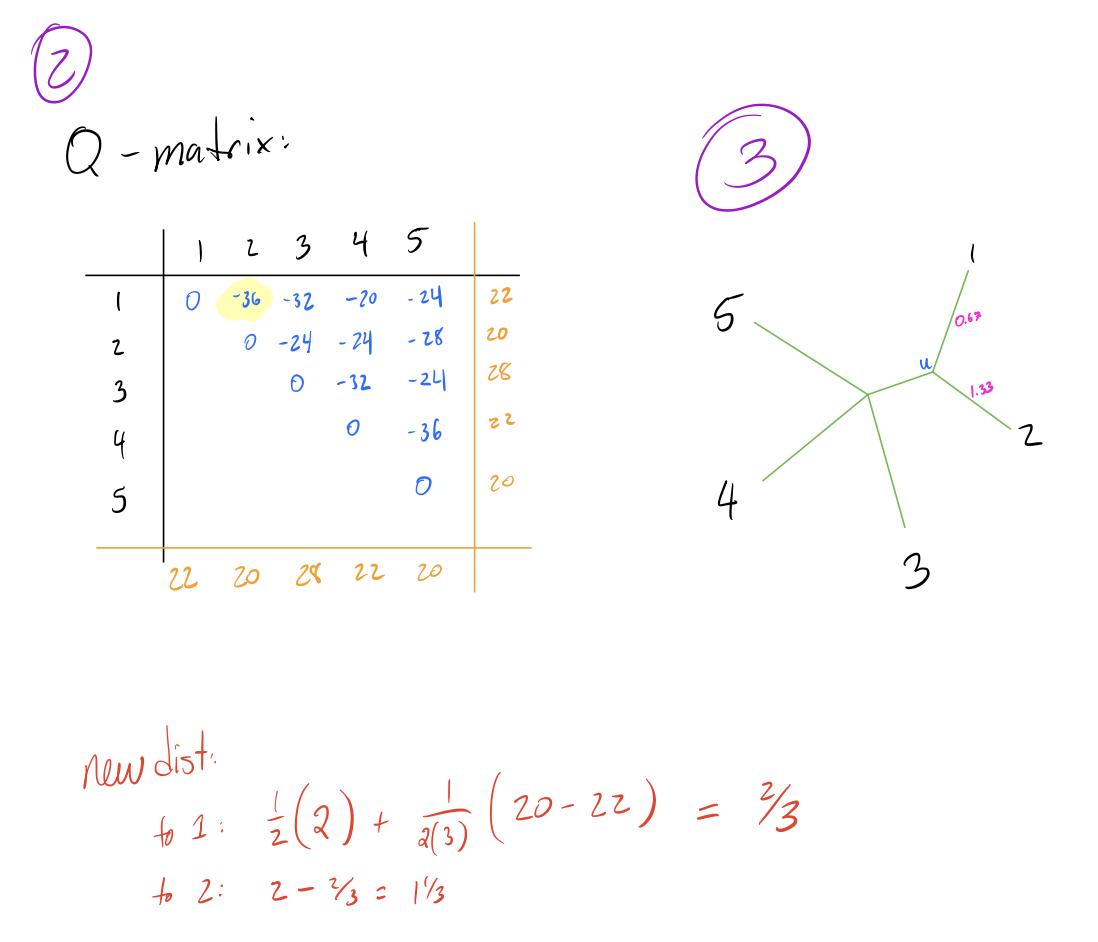
- Calculate edge lengths from \(N_{int}\) to \(f,g\) with the following formula:
\[\begin{align*} d(N_{int}, f) &= \frac{1}{2}(d[i,j]) + \frac{1}{2(n-2)}(R(i) - C(j))\\ \\ d(N_{int}, g) &= d[i,j] - d[N_{int}, f] \end{align*}\]
- Calculate distance from \(N_{int}\) to all other nodes \(h\) with the following formula:
\[d(h, N_{int}) = \frac{1}{2}(d[h,g] + d[h,f] - d[f,g])\]
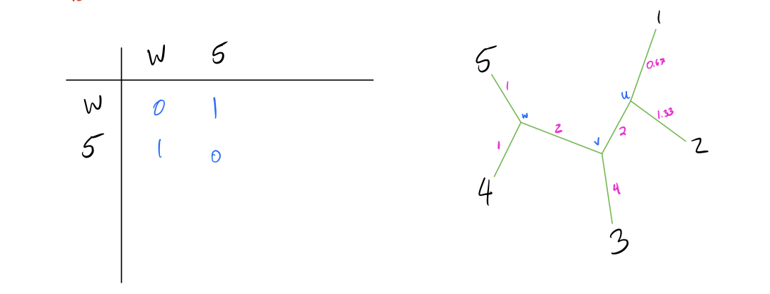
- Repeat until the full tree has been constructed.
branch lengths.
R Implementation
Neighbor-Joining trees can be created R with the following commands. Note that the output is slightly different due to a different method for calculating the initial distance matrix.
dend <- TreeLine(myDistMatrix=dm, method='NJ')
plot_tree_unrooted(dend, 'Neighbor Joining')
Maximum Parsimony Trees
The last way to construct phylogenies that I will discuss is maximum parsimony. This method relies on the assumption that the simplest method is likely the best, and thus tries to find a tree that minimizes the number of changes on the tree. Such a tree is called the most “parsimonious” tree.
Building Initial Tree
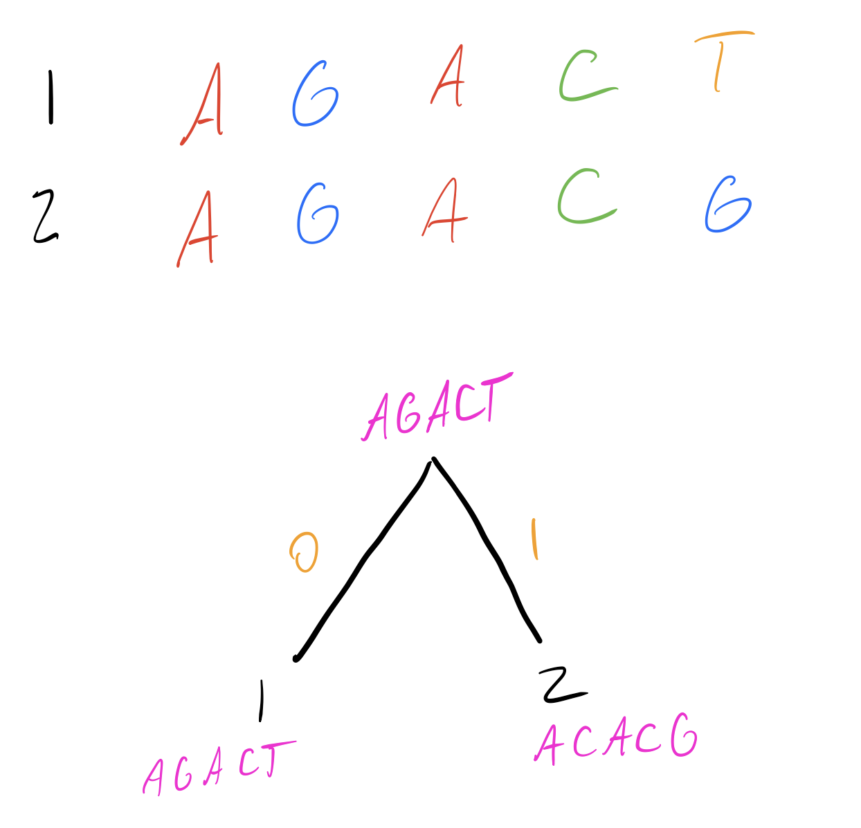
Let’s start by constructing a simple tree between our first two sequences. The intermediate node is labeled with a consensus sequence, which in this case is either sequence 1 or sequence 2. Both are equally parsimonious, since they minimize the total number of transitions on each branch.
I’ve labelled in pink the state at each node, and in orange the number of transitions to go between the nodes connected by that edge.
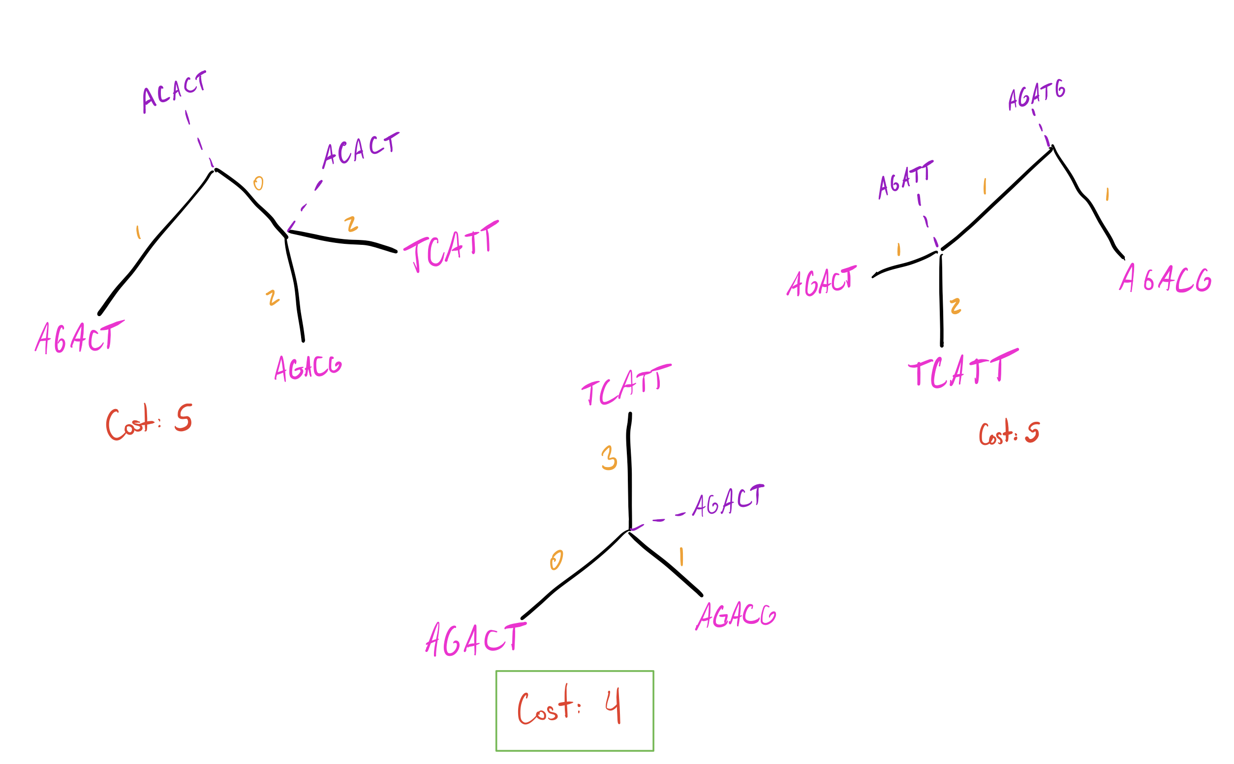
We’ll now add each subsequent sequence. Let’s move on to sequence 3.
There are 3 total ways to add sequence 3 to our tree:
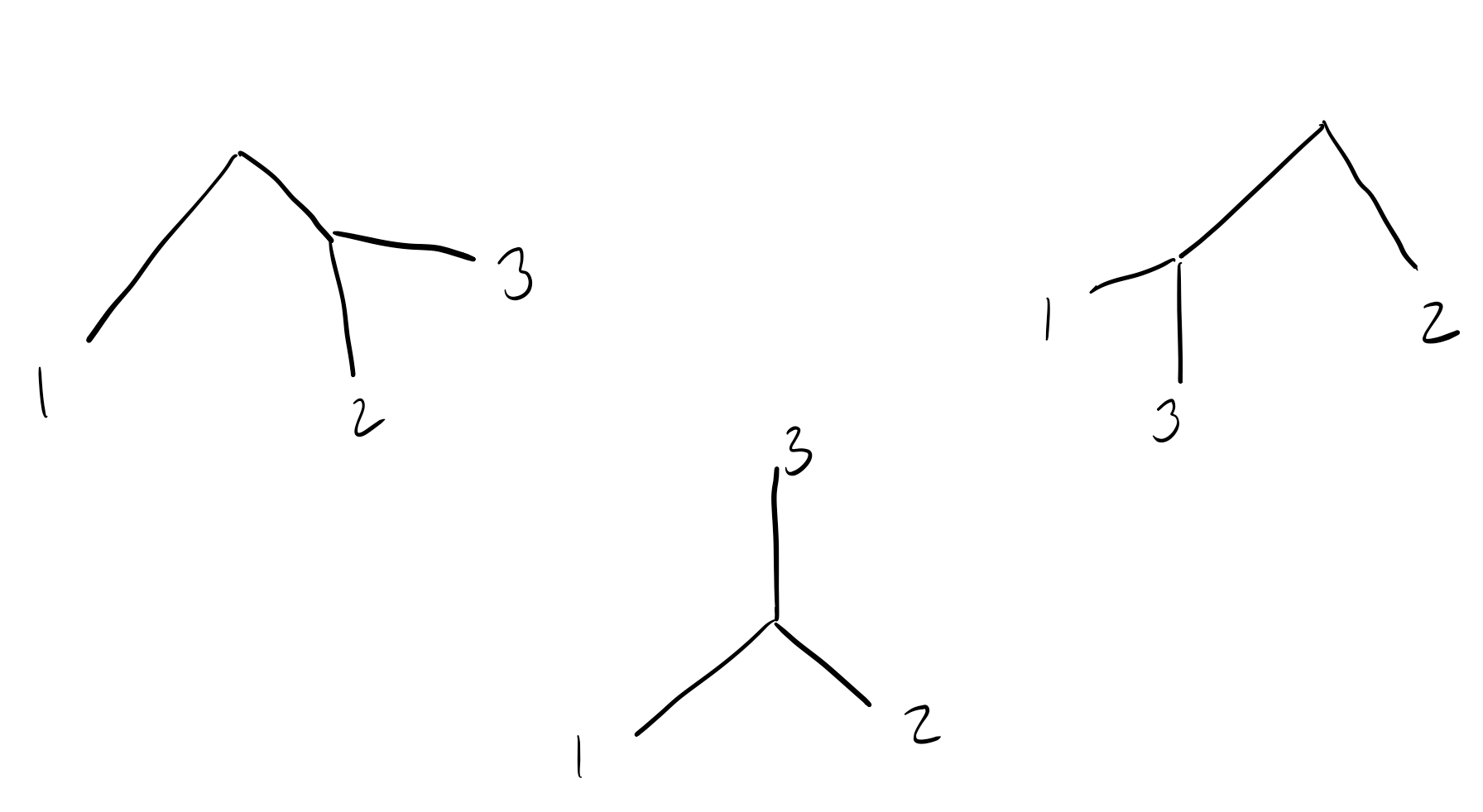
Two of these trees place sequence 3 closer to sequence 1/2 than sequence 2/1 (resp.), and the middle tree places all sequences equally far apart.
Let’s now label these trees with intermediate states and see how parsimonious they are:
Short digression on how we find intermediate/ancestral sequences:
In the middle tree, there is only one choice for the ancestral sequence, which is the one where each position is seen in the majority of sequences. Each position in it (\(AGACT\)) appears in \(2/3\) of nodes connected to it (first position of 1 and 2 is \(A\), second of 1 and 2 is \(G\), etc.). If there were a position where all nodes were different, we would be free to pick any of those bases (since all are equally represented and thus will be equally parsimonious). There are often multiple ways to construct ancestral states, but they should end up being equal. Look into Fitch Parsimony and/or Sankoff Parsimony for a more rigorous definition of how to find parsimonious ancestor states.
Back to the tutorial–the star tree is the most parsimonious! Our tree
now looks like this: 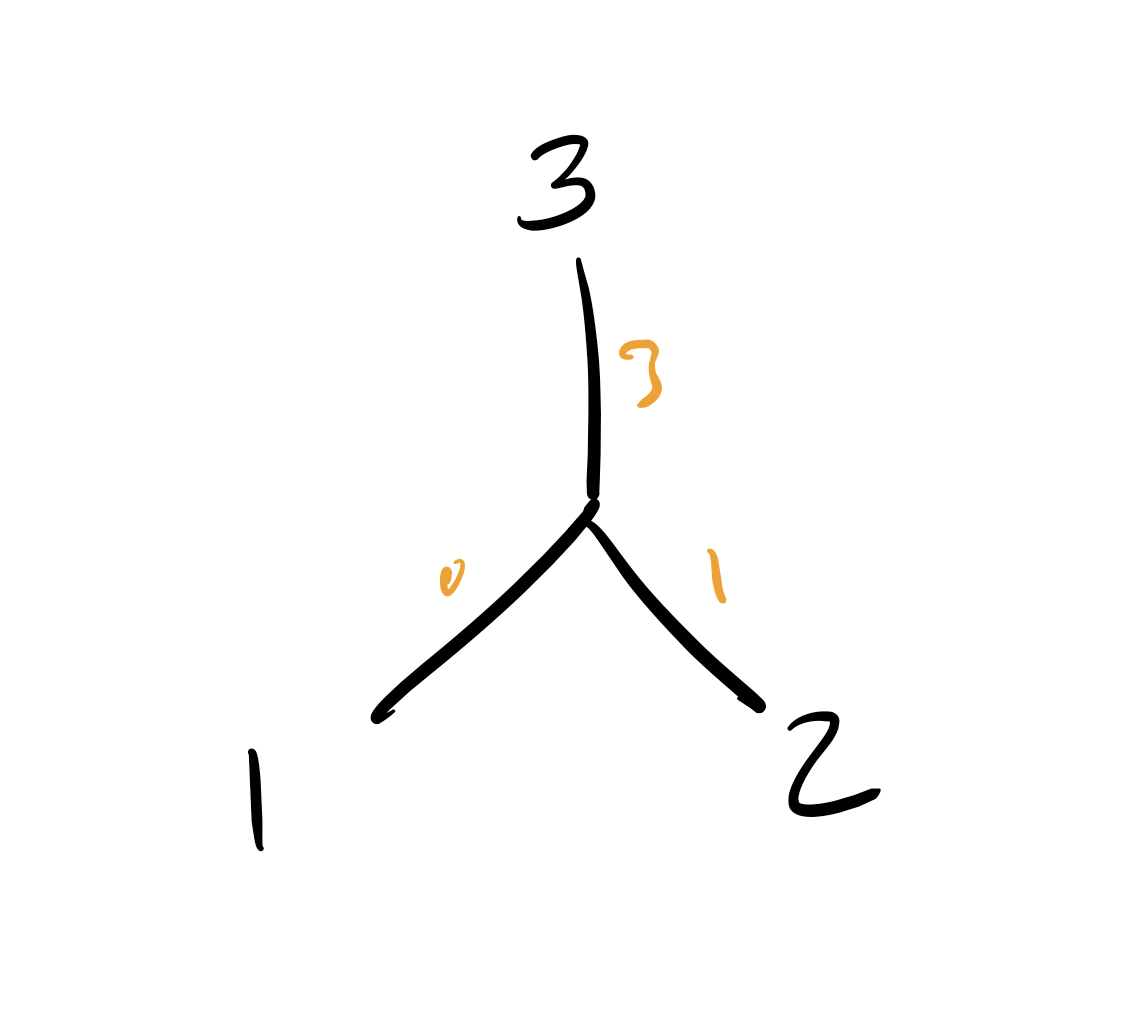
Just to really drive the point home, let’s walk through adding
sequence 4 to the tree. There are now 4 options where we can put this
sequence: 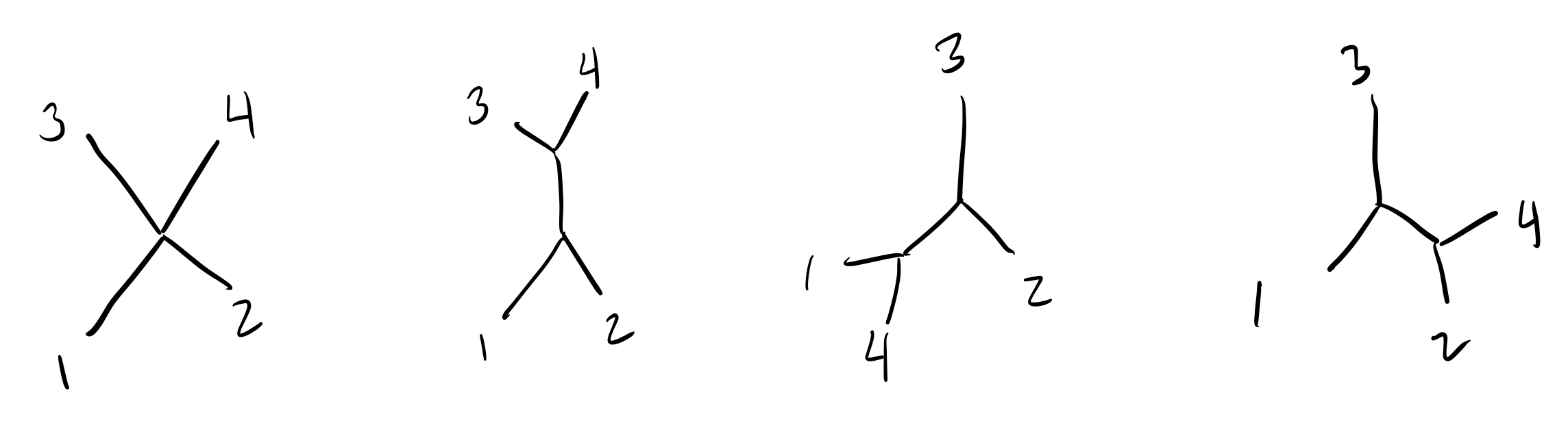
And again filling in ancestral states and finding transitions on each branch:
I’m going to skip walking through adding sequence 5 since it begins to have a lot of possibilities, but suppose we arrive at the following tree after adding sequence 5:
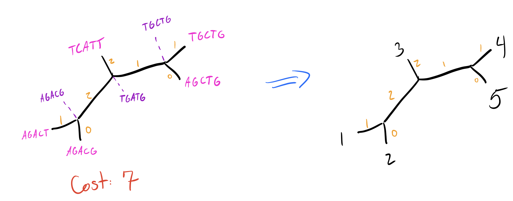
Now we have our initial tree, which has a total parsimony cost of 7. However, we’re not done yet. Adding branches sequentially doesn’t guarantee we get an optimal solution, especially if we incorporate optimizations to how we add branches. Many algorithms commonly only minimize the parsimony cost of the branch at each addition (rather than recalculating the entire tree) to speed up calculations. This can cause us to miss better solutions due to local maxima. One common solution to this is to perturb our initial tree.
Nearest Neighbor Interchanges
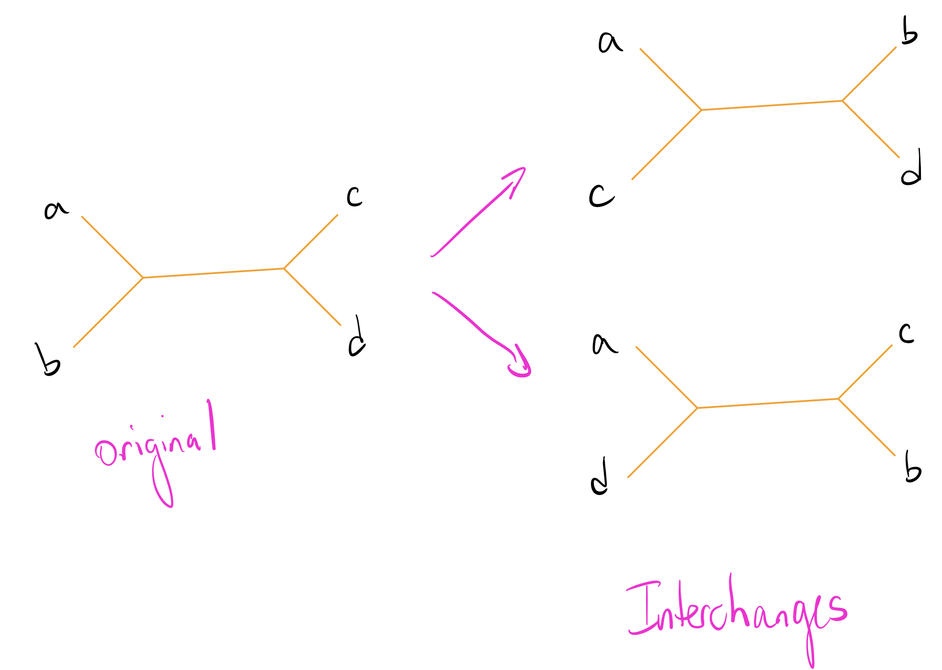
The most common way to perturb a phylogenetic tree is with Nearest Neighbor Interchanges (NNIs). For any particular set of 4 nodes, there are 3 distinct ways to partition them into pairs. An NNI changes this partition and rechecks the parsimony of the result to see if we can get an improvement.
NNIs are significantly easier to explain with images. Suppose we have a set of nodes \(\{a, b, c, d\}\) such that \(a,b\) are separated from \(c,d\). Our possible NNIs then look like this:
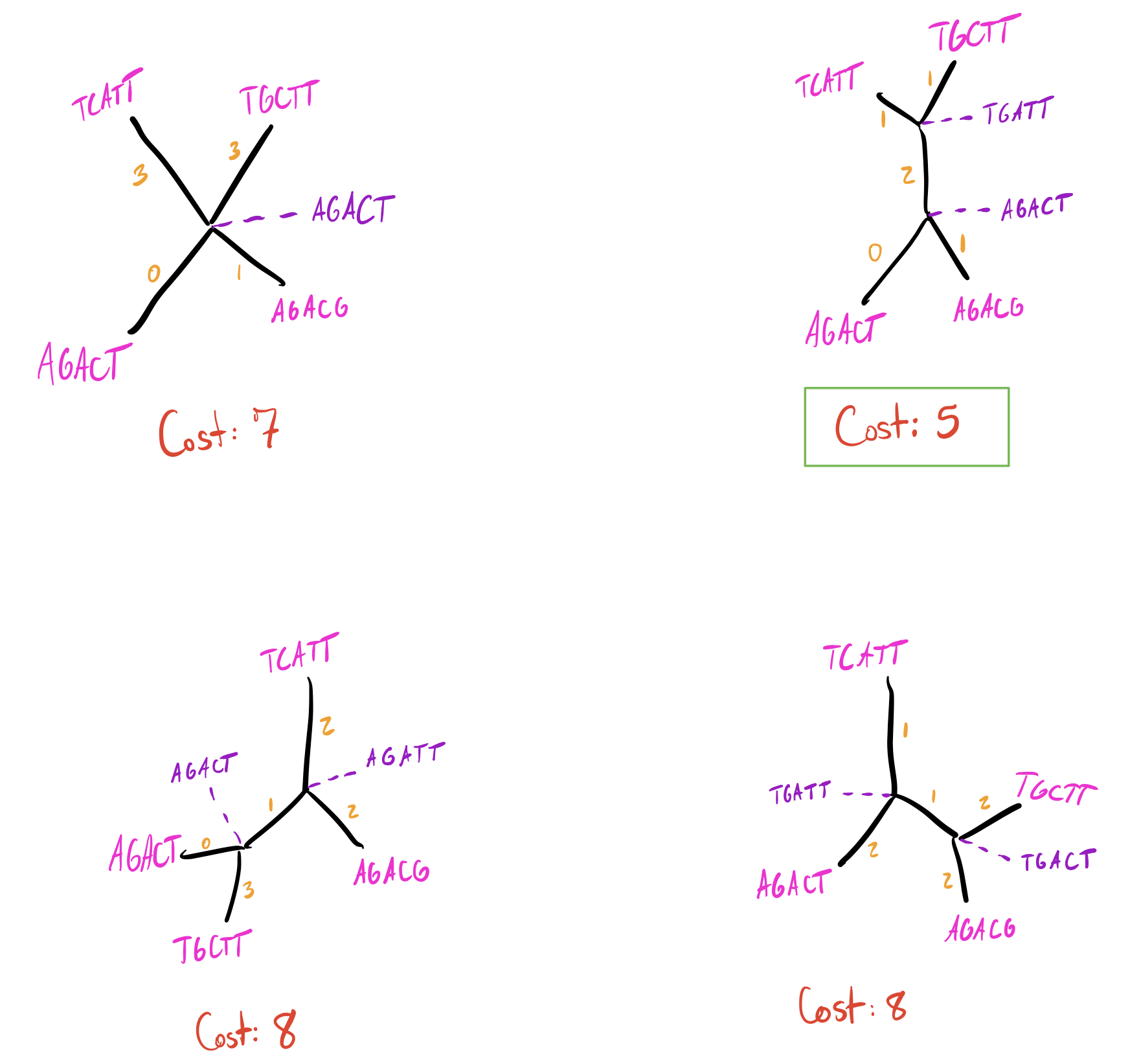
Let’s explore this on our initial tree by making an NNI on the edge that separates \(\{4,5\}\) from the rest of the nodes. We’ll have two trees to check:
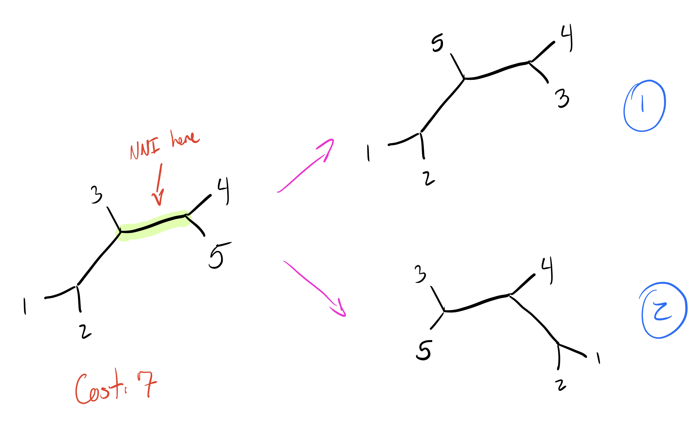
As mentioned above, the total cost for our current tree is 7. Do any of these new trees do better?
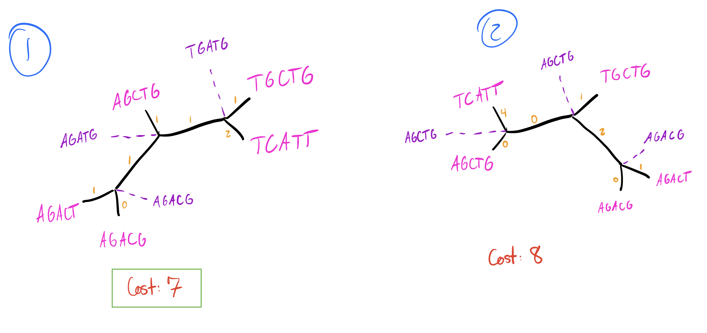
So tree 2 is worse, but tree 1 is just as good as our initial tree! I’m going to skip walking through all the other NNIs on other branches, so let’s look at our final two equally parsimonious reconstructions (node labels blue, branch lengths in orange):
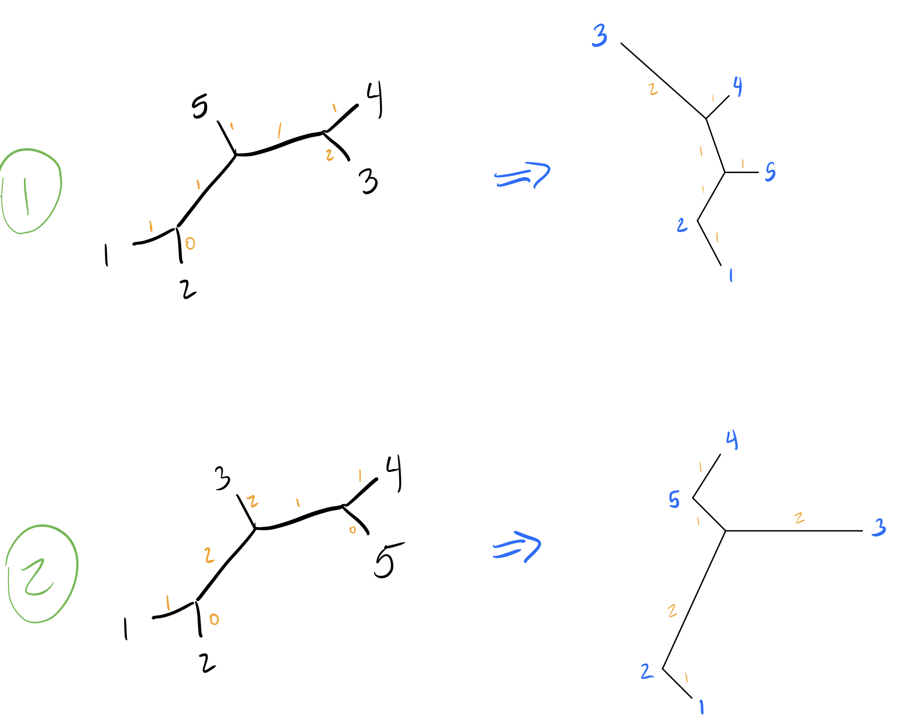
Note that we can remove branches with length 0.
R Implementation
We can do maximum parsimony reconstructions in R using the following code:
dend <- TreeLine(sequenceSet, method='MP')
plot_tree_unrooted(dend, 'Maximum Parsimony')
Notice that this almost exactly matches one of our own reconstructions! Parsimony reconstructions can differ based on how you calculate parsimony, which can account for why the lengths in this plot are slightly different than ours. Using a different transition cost model (such as weighting transitions different than transversions) can lead to different results.