Comparing Trees

Making trees is nice, but how do we compare them? Comparing trees is a difficult problem, since they can contain significantly different topologies.

In this discussion I’ll cover two common ways of calculating distances between trees: Robinson-Foulds (RF) Distance and Kuhner-Felsenstein (KF) distance.

options(rmarkdown.html_vignette.check_title = FALSE)

# Package imports
library(ape)
library(DECIPHER)

# Helper plotting function
plot_tree_unrooted <- function(dend, title){
  tf <- tempfile()
  WriteDendrogram(dend, file=tf, quoteLabels=FALSE)
  predTree <- read.tree(tf)
  plot(predTree, 'unrooted', main=title)
}

Setup

We’ll start with a slightly larger test dataset so that we can more clearly see differences between tree constructions. The following codeblocks read in a set of 25 simulated alignments, then constructs phylogenetic trees using the three methods discussed previously.

# External data file, contains simulated alignment
simSeqsFile <- system.file('extdata', 'Simulated_v1.fas', package='LakshmanTutorials', mustWork=TRUE)

simAli <- suppressWarnings(readDNAStringSet(simSeqsFile))[1:25]
names(simAli) <- 1:25
simDm <- DistanceMatrix(simAli, type='dist', verbose=FALSE)

UPGMAtree <- as.dendrogram(hclust(simDm, method='average'))
NJtree <- TreeLine(simAli, myDistMatrix=simDm, method='NJ')
MPtree <- TreeLine(simAli, myDistMatrix=simDm, method='MP')

Visualizing the trees we’ve made:

plot_tree_unrooted(UPGMAtree, 'UPGMA')

plot_tree_unrooted(NJtree, 'NJ')

plot_tree_unrooted(MPtree, 'MP')

Partitions

Before we dive into tree distances, it’s important to understand the concept of partitions. In a bifurcating unrooted tree, every edge divides the set of leaf nodes into two sets. These form the basis of many tree comparison algorithms. Let’s look at a toy example:

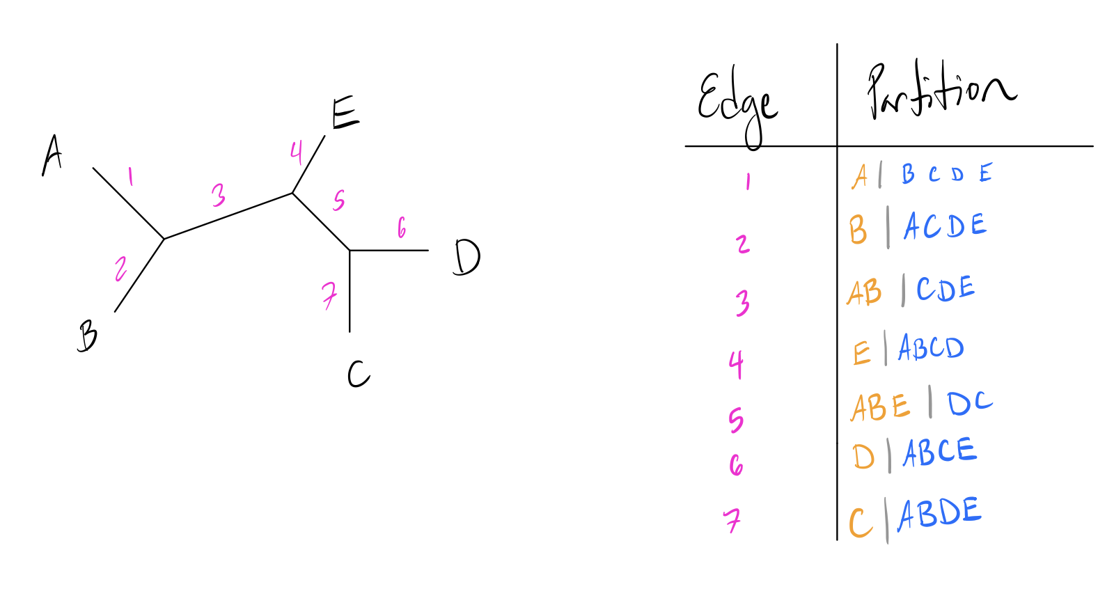
Note how each numbered edge of the tree splits the labeled leaf nodes into two distinct groups to either side of it. Leaf edges trivially split the tree into a partition of just the leaf and everything else, but internal edges split the leaves into more interesting partitions.

RF Distance

Robinson-Foulds (RF) distance measures the similarity of these partitions in a tree. Let’s look at a toy example with two small trees and their internal partitions labeled (internal edges circled in green):

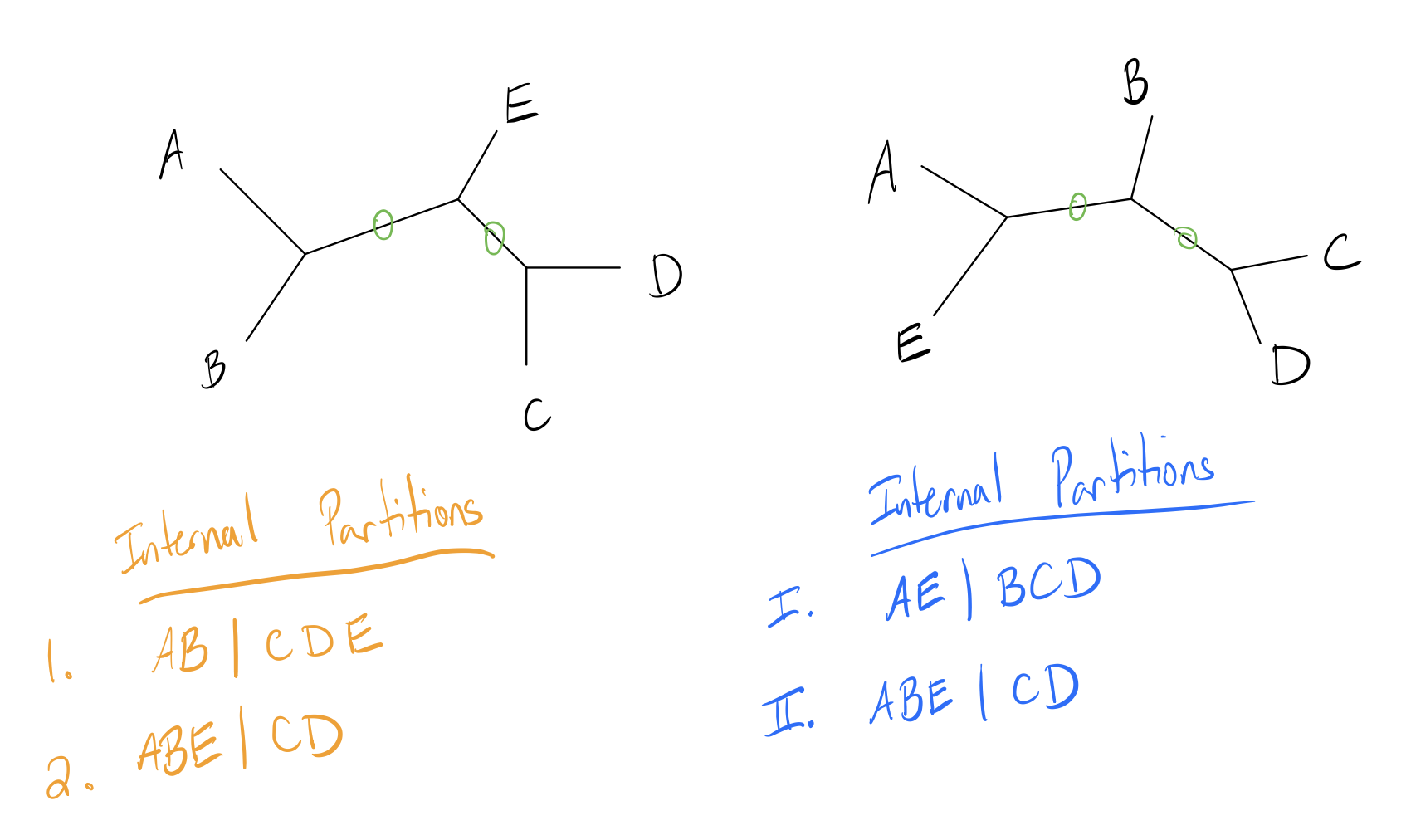
Now let \(A\) be the number of partitions unique to the first tree, and \(B\) the number of partitions unique to the second tree. The RF distance (also called the symmetric difference metric) is simply the quantity \((A+B)\).

For this example, note that edge 2 is an identical partition to edge II. Thus, the first tree has one unique partition, and the second tree has one unique partition, so the RF distance is \(1+1=2\).

Some implementations change the metric slightly by scaling it, either by dividing by two or scaling the metric to have a maximum value of 1. The latter operation can be done by dividing by the maximum possible score, which is just the sum of the total number of branches. In this case, the total number of internal branches is 4 (2 from each tree), so the RF distance is \(0.5\).

R implementation

RF_dist_external <- function(dend1, dend2){
  tf <- tempfile()
  WriteDendrogram(dend1, file=tf, quoteLabels=FALSE)
  predTree1 <- read.tree(tf)
  
  tf <- tempfile()
  WriteDendrogram(dend2, file=tf, quoteLabels=FALSE)
  predTree2 <- read.tree(tf)
  
  return(dist.topo(predTree1, predTree2, 'PH85'))
}

RF_dist_external(UPGMAtree, NJtree)

##       tree1
## tree2    12

RF_dist_external(UPGMAtree, MPtree)

##       tree1
## tree2    18

RF_dist_external(NJtree, MPtree)

##       tree1
## tree2    12

Drawbacks

RF distance is widely used, but has some common issues that should be kept in mind while using it:

Lacks sensitivity
- Similar trees can receive the same value
- Range of values depends on tree shape
- Doesn’t look at branch length
Can’t recognize similar clades (any difference increases distance score)
Original implementation assumes bifurcating, unrooted tree with same leaf set
Distance is not immediately statistically interpretable (larger \(\neq\) significant)

Some of these drawbacks have been accounted for with subsequent optimization, and ‘generalized RF distances’ have been created that can account for similar sets while working on multifurcating trees with different leaf sets.

KF Distance

The Kuhner-Felsenstein (KF) distance attempts to incorporate branch lengths into the RF distance to gain a richer description of the differences between two trees.

Recall that the RF distance is the number of unique (non-shared) partitions in the tree. The KF distance is instead taken as the sum of the squared difference of branch lengths for each equivalent partition in the two trees. If a partition is a unique to a particular tree, it is taken as having a branch length of 0 in the other tree. Below is an updated version of our previous example with branch lengths added in pink (partitions labeled):

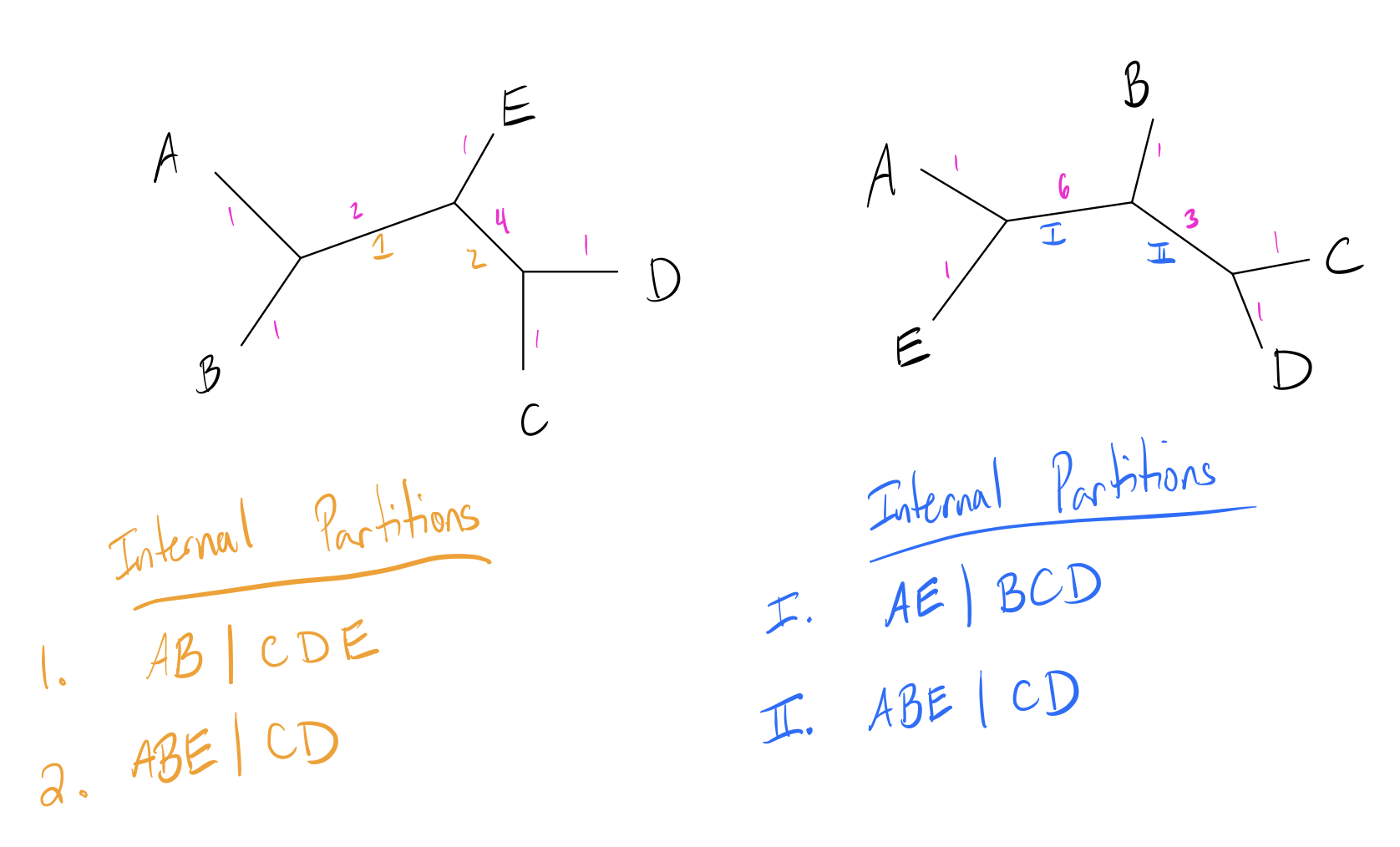
Here we will also examine the leaf branches, but since the leaf set is the same and branch lengths are identical, all of these branches cancel each other out. One pair of branches is an equivalent partition (2 and II), and the other two are unique. The KF distance is then:

\[\begin{align*} KF(Tr1, Tr2) &= (len(1) - 0)^2 + (0 - len(I))^2 + (len(2) - len(II))^2 \\ &= (2-0)^2 + (0-6)^2 + (2-3)^2 \\ &= 41 \end{align*}\]

The advantages of this over RF distance is that it can incorporate branch lengths in addition to topology, which allows it to downweight small differences in topology and upweight large differences.

R Implementation

KF_dist_external <- function(dend1, dend2){
  tf <- tempfile()
  WriteDendrogram(dend1, file=tf, quoteLabels=FALSE)
  predTree1 <- read.tree(tf)
  
  tf <- tempfile()
  WriteDendrogram(dend2, file=tf, quoteLabels=FALSE)
  predTree2 <- read.tree(tf)
  
  return(dist.topo(predTree1, predTree2, method='score'))
}

RF_dist_external(UPGMAtree, NJtree)

##       tree1
## tree2    12

RF_dist_external(UPGMAtree, MPtree)

##       tree1
## tree2    18

RF_dist_external(NJtree, MPtree)

##       tree1
## tree2    12

Generalized Robinson-Foulds Distance

As mentioned before, RF distance has a number of drawbacks. Correcting these has led to a family of metrics referred to as “Generalized Robinson-Foulds Distances”. These metrics attempt to measure differences in partitions not as binary values, but as continuous measures to incorporate how different a given partition is from another. Two of the most successful of these measures are the information-theoretic generalized RF Distance measures, Phylogenetic Information Content and Mutual Clustering Information. Description of these metrics is sourced from Smith (2020).

RF Distance always operates on partitions. Let a given partition be defined as \(S = A|B\), where \(A\) and \(B\) are disjoint leaf sets. In classic RF Distance, if we have an \(S\) such that no identical \(S\) exists in the other tree, we add one to the distance.

Phylogenetic Information Content

In Phylogenetic Information Content, we instead score each pair of partitions using the probability we would encounter a similar partition by chance. For a given set of \(n\) genomes, there are \((2n-5)!!\) possible unrooted binary trees. Here \(x!!\) is the double factorial, defined as \(x!! = x * (x-2)!!\) with \(1!!=0!!=1\). Then for a given pair of splits \(S_1 = A_1|B_1\) and \(S_2 = A_2|B_2\) on a tree with \(n\) leaves, the probability of a randomly chosen binary tree containing these two splits is then:

\[\begin{align*} P(S_1,S_2) = \frac{(2(|B_1|+1)-5)!!(2(|A_2|+1)-5)!!(2(|A_1|-|A_2|+2)-5)!!}{(2n-5)!!} \end{align*}\]

To obtain shared phylogenetic information, for each pair of splits we set \(h = 0\) if \(S_1\) and \(S_2\) conflict, and \(h(S_1) + h(S_2) + h(S_1,S_2)\) with \(h(S_1,S_2) = -\log(P(S_1,S_2))\). Summing this value across an optimal pairing of nodes results in the Shared Phylogenetic Information Score.

Mutual Clustering Information

Mutual Clustering Information is similar to Shared Phylogenetic Information in that it quantifies the similarity of a given partition, but this metric instead uses mutual information of the partition rather than a p-value-like measure.

Let \(P(A) = \frac{|A|}{n}\), and \(P(A_1,A_2) = \frac{|A_1 \cap A_2|}{n}\). Then the mutual clustering information between two splits \(S_1 = A_1|B_1\) and \(S_2 = A_2|B_2\) is given as:

\[\begin{align*} I(S_1, S_2) = P(A_1,A_2)\log&\frac{P(A_1,A_2)}{P(A_1)P(A_2)} + P(A_1,B_2)\log\frac{P(A_1,B_2)}{P(A_1)P(B_2)} + \\ &P(B_1,A_2)\log\frac{P(B_1,A_2)}{P(B_1)P(A_2)} + P(B_1,B_2)\log\frac{P(B_1,B_2)}{P(B_1)P(B_2)} \end{align*}\]

The individual entropy of a given split \(h(S)\) is given as \(-[P(A)\log P(A) +P(B)\log P(B)]\). Summing \(I\) over an optimal pairing of splits produces the mutual clustering information score. This can be converted into a distance by taking:

\[\begin{align*} CID = \frac{\sum_{S_1 \in T_1} h(S_1) + \sum_{S_2 \in T_2} h(S_2) - \sum_{(s_1,s_2) \in Pairing} I(s_1, s_2)}{\sum_{S_1 \in T_1} h(S_1) + \sum_{S_2 \in T_2} h(S_2)} \end{align*}\]

Where \(S_i \in T_i\) is the splits in the first tree and \(Pairing\) is an optimal pairing of splits between the two trees.

R Implementation

library(SynExtend)

GeneralizedRF(UPGMAtree, NJtree)
GeneralizedRF(UPGMAtree, MPtree)
GeneralizedRF(NJtree, MPtree)

Other Metrics

These are two commonly used metrics, but many more are implemented in the TreeDist package. Notable other tree distance measures include:

Jaccard-Robinson-Foulds: Generalized RF distance similar to CMI, but using Jaccard Distance of the splits rather than mutual information.
- (Böcker et al., 2013)
Path Difference Metric: Euclidean distance of the vector formed from taking the upper triangle of the Cophenetic Distance matrices.
- (Steel and Penny, 1993)
MAST(I): Maximal Agreeing SubTree of the two trees. MAST looks at the number of leaves in this tree, whereas MASTI uses phylogenetic information content.
- (MAST: Kao et al., 2001; MASTI: Smith 2020a).
Subtree Prune and Regraft (SPR) Distance: number of SPR operations required to transform one tree into another.
- (Hein 1990)
Quartet Divergence: number of quartets that agree between the two trees.
- (Estabrook et al., 1985)
Nearest Neighbor Interchange (NNI) distance: measuring how many NNIs are required to transform one tree into another.
- (Li et al., 1996)

A comprehensive evaluation of many of these metrics is available in this paper.

Manual Implementations

I wrote implementations of RF, KF, and GRF distances from scratch to illustrate how these functions are working under the hood. Note that external packages incorporate some optimizations for RF/KF I didn’t implement that lead to different results. The best of these is GeneralizedRF(), available through SynExtend (not shown here since it is significantly longer than the other two methods).

Helper functions

This code block contains several helper functions used later.

flatdendrapply <- function(dend, NODEFUN, LEAFFUN=NODEFUN, INCLUDEROOT=TRUE, ...){
  ## Applies a function to each node (internal and leaf) of the tree
  ## Returns a flat list
  val <- lapply(dend, 
                \(x){
                  if (is.null(attr(x, 'leaf'))){
                    v <- list(NODEFUN(x, ...))
                    for ( child in x ) v <- c(v, Recall(child))
                    return(v)
                  } 
                  else if (!is(LEAFFUN, 'function'))
                    return(list())
                  else 
                    return(list(LEAFFUN(x, ...)))
                }
  )
  retval <- unlist(val, recursive=FALSE)
  if (!INCLUDEROOT)
    retval[[1]] <- NULL

  return(retval)
}

isLeaf <- function(dendNode){
  return(!is.null(attr(dendNode, 'leaf')) && attr(dendNode, 'leaf'))
}

equivPart <- function(set1, set2, fullset){
  # Checks if two partitions are equivalent
  inverseset1 <- fullset[!(fullset %in% set1)]
  return(setequal(set1,set2) || setequal(inverseset1, set2))
}

get_branch_length <- function(dendNode){
  ## Helper function for KF distance, gets partition and branch length
  ## of all branches Because of weirdness each node will return two values,
  ## the result just needs some slight post-processing 
  ## (see KF_Distance function for example)
  if(isLeaf(dendNode)){
    return(0)
  }
  
  h <- attr(dendNode, 'height')
  n1 <- dendNode[[1]]
  n2 <- dendNode[[2]]
  c1 <- attr(n1, 'height')
  c2 <- attr(n2, 'height')
  
  if(isLeaf(n1))
    labs1 <- attr(n1, 'label')
  else 
    labs1 <- unlist(n1)
  
  if (isLeaf(n2))
    labs2 <- attr(n2, 'label')
  else
    labs2 <- unlist(n2)

  l1 <- list(length=h-c1, part=labs1)
  l2 <- list(length=h-c2, part=labs2)
  return(list(l1, l2))
}

Robinson-Foulds Distance

RF_Distance <- function(dend1, dend2){
  # Get all partitions
  part1 <- flatdendrapply(dend1, unlist, NULL)
  part2 <- flatdendrapply(dend2, unlist, NULL)
  allmembers <- unique(c(unlist(dend1), unlist(dend2)))
  
  # Calculate tree distance
  A <- B <- 0
  for ( i in seq_along(part1))
    A <- A + !any(sapply(part2, \(x) equivPart(part1[[i]], x, allmembers)))
  
  for ( i in seq_along(part2))
    B <- B + !any(sapply(part1, \(x) equivPart(part2[[i]], x, allmembers)))
  
  # This implementation normalizes to get a distance out of 1
  return((A+B) / (length(part1) + length(part2)))
}

Kuhner-Felsenstein Distance

KF_Distance <- function(dend1, dend2){
  # Get all branch lengths and partitions
  part1 <- flatdendrapply(dend1, get_branch_length, NULL)
  part2 <- flatdendrapply(dend2, get_branch_length, NULL)
  
  # Each function call returns a length of list two, we just want the members
  part1 <- unlist(part1, recursive=FALSE)
  part2 <- unlist(part2, recursive=FALSE)
  
  # Root is split into two branches, need to combine
  part1[[1]]$length <- part1[[1]]$length + part1[[2]]$length
  part2[[1]]$length <- part2[[1]]$length + part2[[2]]$length
  part1[[2]] <- part2[[2]] <- NULL
  
  allmembers <- unique(c(unlist(dend1), unlist(dend2)))
  
  # For each
  treedist <- 0
  for ( i in seq_along(part1)){
    check <- sapply(part2, \(x) equivPart(part1[[i]]$part, x$part, allmembers))
    if (any(check)){
      loc <- which(check)
      treedist <- treedist + (part1[[i]]$length - part2[[loc]]$length)**2
    }
  }
  for ( i in seq_along(part2)){
    check <- sapply(part1, \(x) equivPart(part2[[i]]$part, x$part, allmembers))
    if (any(check)){
      loc <- which(check)
      treedist <- treedist + (part2[[i]]$length - part1[[loc]]$length)**2
    }
  }
  
  ## divided by two since duplicates will be added twice
  ## probably worth reworking at some point to avoid adding duplicates twice,
  ## this is just a quick fix
  return(sqrt(treedist/2))
}

Generalized RF Distance

GRF <- function(dend1, dend2){
  require(SynExtend)
  return(GeneralizedRF(dend1, dend2))
}

Comparison

RFDists <- KFDists <- GRFDists <- matrix(0, nrow=3, ncol=3)
rownames(RFDists) <- rownames(KFDists) <- rownames(GRFDists) <-
  colnames(RFDists) <- colnames(KFDists) <- colnames(GRFDists) <-
  c('UPGMA', 'NJ', 'MP')

RFDists[1,2] <- RFDists[2,1] <- RF_Distance(UPGMAtree, NJtree)
RFDists[1,3] <- RFDists[3,1] <- RF_Distance(UPGMAtree, MPtree)
RFDists[2,3] <- RFDists[3,2] <- RF_Distance(NJtree, MPtree)
KFDists[1,2] <- KFDists[2,1] <- KF_Distance(UPGMAtree, NJtree)
KFDists[1,3] <- KFDists[3,1] <- KF_Distance(UPGMAtree, MPtree)
KFDists[2,3] <- KFDists[3,2] <- KF_Distance(NJtree, MPtree)
#GRFDists[1,2] <- GRFDists[2,1] <- GRF(UPGMAtree, NJtree)
#GRFDists[1,3] <- GRFDists[3,1] <- GRF(UPGMAtree, MPtree)
#GRFDists[2,3] <- GRFDists[3,2] <- GRF(NJtree, MPtree)

RFDists

##           UPGMA        NJ        MP
## UPGMA 0.0000000 0.2608696 0.3913043
## NJ    0.2608696 0.0000000 0.2608696
## MP    0.3913043 0.2608696 0.0000000

KFDists

##           UPGMA        NJ        MP
## UPGMA 0.0000000 0.9712953 1.0367032
## NJ    0.9712953 0.0000000 0.3419947
## MP    1.0367032 0.3419947 0.0000000

#GRFDists

Aidan Lakshman1

Setup

Partitions

RF Distance

R implementation

Drawbacks

KF Distance

R Implementation

Generalized Robinson-Foulds Distance

Phylogenetic Information Content

Mutual Clustering Information

R Implementation

Other Metrics

Manual Implementations

Helper functions

Robinson-Foulds Distance

Kuhner-Felsenstein Distance

Generalized RF Distance

Comparison

Aidan Lakshman¹