Building Coevolution Networks with SynExtend

Aidan Lakshman¹

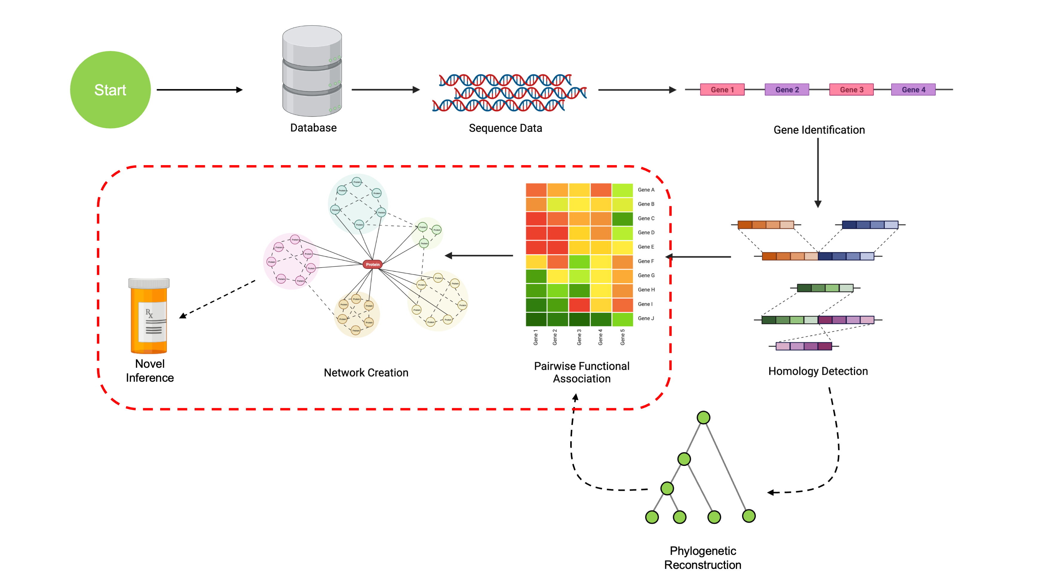
Coevolutionary Analysis

At this point, we’ve walked through the steps to take a set of sequences and obtain a set of COGs with phylogenetic reconstructions for each COG. We’re now ready to look for signals of coevolution, which imply functional associations between COGs. These methods are implemented via the EvoWeaver class in SynExtend, which includes many commonly used methods for detecting coevolutionary patterns.

While the previous steps have only utilized a small subsample of the data, we’re now finally going to work with the complete dataset. This dataset is comprised of the 91 Micrococcus genomes available with assemblies at the Scaffold, Chromosome, or Complete level (link to query). Note that more genomes may become available after this conference; these are all that were available at the time.

We ran the complete pipeline of identifying and annotating genes with DECIPHER, finding COGs with SynExtend, and then creating gene trees for each COG using DECIPHER. The complete data consist of 3,407 distinct COGs. All of this analysis is performed entirely within SynExtend and DECIPHER; no external packages or data are required aside from the input genomes.

We now use the new EvoWeaver class to try to find COGs that show evidence of correlated evolutionary selective pressures, also referred to as ‘coevolutionary signal’.

Download Complete Micrococcus Dataset

 

library(DECIPHER)
library(SynExtend)

COGsFile <- '/path/to/MicrococcusCOGs.RData'
AnnotationsFile <- '/path/to/MicrococcusAnnotations.RData'
TreesFile <- '/path/to/MicrococcusGeneTrees.RData'

# All of these files are formatted the same way, as lists with each entry
# corresponding to a COG. COGs entries are identifiers for each gene, CogsAnnot 
# entries are annotations, and CogTrees entries are gene trees
load(COGsFile)          # Loads 'COGs'
load(AnnotationsFile)   # Loads 'CogsAnnot'
load(TreesFile)         # Loads 'CogTrees'

# Let's look at one of the COGs
COGs[[7]]

##  [1] "1_1_919"     "12_44_1601"  "13_5_415"    "2_1_10"      "14_1_274"   
##  [6] "15_1_14"     "16_132_1767" "17_107_1177" "18_1_1825"   "19_1_1783"  
## [11] "20_1_958"    "21_223_1464" "22_44_1726"  "23_13_736"   "3_1_130"    
## [16] "24_11_767"   "25_1_915"    "26_8_258"    "27_53_1567"  "28_10_1132" 
## [21] "29_53_1900"  "30_1_72"     "31_7_808"    "32_7_458"    "33_183_1337"
## [26] "34_130_2076" "35_197_1194" "36_128_792"  "37_22_1142"  "38_81_1984" 
## [31] "4_1_9"       "39_1_1608"   "40_1_416"    "41_1_925"    "42_1_1032"  
## [36] "43_1_707"    "44_1_704"    "45_13_755"   "46_63_1530"  "47_1_970"   
## [41] "48_1_690"    "49_1_779"    "50_1_267"    "51_20_1253"  "52_1_971"   
## [46] "53_105_395"  "54_109_577"  "55_33_1488"  "56_11_533"   "57_161_2179"
## [51] "58_111_515"  "59_55_1658"  "5_1_9"       "60_50_1995"  "61_1_78"    
## [56] "62_8_204"    "63_155_1042" "64_47_712"   "65_96_2144"  "66_11_774"  
## [61] "67_66_1831"  "68_22_82"    "69_22_1206"  "70_34_781"   "71_96_2235" 
## [66] "72_1_1811"   "73_11_821"   "74_1_221"    "75_15_1093"  "76_1_2110"  
## [71] "77_1_696"    "78_1_1963"   "79_12_872"   "80_12_855"   "81_48_2136" 
## [76] "82_41_671"   "83_20_1289"  "84_185_549"  "85_42_1351"  "86_8_1238"  
## [81] "88_7_611"    "89_126_1611" "90_1_980"    "6_21_1244"   "7_40_2015"  
## [86] "8_1_348"     "9_5_575"     "10_1_382"    "11_1_10"     "11_12_1037" 
## [91] "91_1_985"

CogsAnnot[[7]]

##   A test set of class 'Taxa' with length 91
##      confidence name                 taxon
##  [1]       100% 50_1_267             Root; 09120 Genetic Information Processi...
##  [2]       100% 51_20_1253           Root; 09120 Genetic Information Processi...
##  [3]       100% 52_1_971             Root; 09120 Genetic Information Processi...
##  [4]        71% 53_105_395           Root; 09120 Genetic Information Processi...
##  [5]       100% 54_109_577           Root; 09120 Genetic Information Processi...
##  ...        ... ...                  ...
## [87]       100% 45_13_755            Root; 09120 Genetic Information Processi...
## [88]       100% 46_63_1530           Root; 09120 Genetic Information Processi...
## [89]       100% 47_1_970             Root; 09120 Genetic Information Processi...
## [90]       100% 48_1_690             Root; 09120 Genetic Information Processi...
## [91]       100% 49_1_779             Root; 09120 Genetic Information Processi...

CogsAnnot[[7]][[1]]

## $taxon
## [1] "Root"                                                             
## [2] "09120 Genetic Information Processing"                             
## [3] "09122 Translation"                                                
## [4] "03010 Ribosome [PATH:ko03010]"                                    
## [5] "K02899  RP-L27, MRPL27, rpmA, large subunit ribosomal protein L27"
## 
## $confidence
## [1] 100 100 100 100 100

CogTrees[[7]]

## 'dendrogram' with 2 branches and 91 members total, at height 0.3813559

# Removing leaf labels because they make it hard to read
plot(CogTrees[[7]], leaflab='none', main='COG 7')

There is a ton of data here, and we unfortunately don’t have time to look at all of it. To demonstrate some of the things we can do with EvoWeaver, we’re going to look at subset of the data that is easier to investigate.

We’ll subset the COGs to ones that meet the following characteristics:

• COGs with no paralogs
• COGs not part of the core genome
• COGs present in at least 5 genomes (not singletons or super rare ones)
• COGs with at least one high confidence annotation
• COGs that imply a coding region

These are relatively arbitrary requirements, but they subset the data to an example that runs quickly and is easily understandable. This essentially takes a group of COGs that are not essential to the organisms but tend to appear a lot, that have been characterized individually before.

## Subsetting COGs

# Cutoff values (91 genomes total!)
CoreCutoff <- 88
UnderCutoff <- 5

# Get assembly identifiers for each COG
truncCOGs <- lapply(COGs, \(x) sort(as.integer(gsub('^([0-9]+)_.*', '\\1', x))))

# Find COGs without paralogs
noParas <- sapply(truncCOGs, \(x) length(x) == length(unique(x)))

# Get non-core genome
notCoreCOGs <- sapply(truncCOGs, \(x) length(unique(x)) < CoreCutoff)

# Get genes in more than 5 organisms
notSingles <- sapply(truncCOGs, \(x) length(unique(x)) > UnderCutoff)

# Make sure COGs are coding elements
codingCOGs <- sapply(CogsAnnot, \(x) is(x, 'Taxa'))

# At least one high confidence annotation
highConf <- sapply(CogsAnnot, \(x) 
                   if(is(x, 'Taxa')) 
                     max(sapply(x, \(y) 
                                y$confidence[length(y$confidence)])) > 50
                   else FALSE
                   )

# Subset for the workshop
WorkshopSubset <- noParas & notCoreCOGs & notSingles & codingCOGs & highConf

# Subset our data
WCogs <- COGs[WorkshopSubset]
WAnnots <- CogsAnnot[WorkshopSubset]
WTrees <- CogTrees[WorkshopSubset]

Let’s also put together a list of consensus annotations for each COG.

# Initialize a character vector to populate
consAnnots <- vector('character', length=length(CogsAnnot))

# Loop along the annotations for each COG
for ( i in seq_along(CogsAnnot) ) {
  taxaentry <- CogsAnnot[[i]]
  
  # If no annotation, it's a noncoding gene
  if (!is(taxaentry, 'Taxa'))
    consAnnots[[i]] <- 'NONCODING'
  # Otherwise it's a coding gene
  else {
    # Grab all the annotations aside from "Unclassified"
    annots <- sapply(taxaentry, \(y) y$taxon[length(y$taxon)])
    annots <- annots[annots!='unclassified_Root']
    
    # If we only have "Unclassified", just mark it as uncharacterized
    if (length(annots) == 0)
      consAnnots[[i]] <- 'Uncharacterized'
    
    # Otherwise take the most common annotation
    else
      consAnnots[[i]] <- names(sort(table(annots), decreasing=T))[1]
  }
}

Now we can make our EvoWeaver object. EvoWeaver has multiple input options, either a list formatted like COGs (list with gene identifiers) or a list like CogTrees (list with gene trees).

# EvoWeaver constructor
pw <- EvoWeaver(WTrees)

The EvoWeaver constuctor automatically detects the type of data you have and adjusts available predictors accordingly. While it functions best with a list of dendrograms for each COG, it can also run with simple presence/absence patterns. See the documentation file for EvoWeaver for more information on this functionality.

We’re now ready to make predictions. Predicting functional associations is done with the predict.EvoWeaver S3 method. Let’s examine possible functional associations between the COGs we have.

preds <- predict(pw)

print(preds)

##          116   292   303   323   349   357   457   489   490         3336  
##     116  1.00  0.30  0.20  0.22  0.26  0.31  0.20  0.26  0.26     ⋯  0.35 
##     292        1.00  0.17  0.28  0.23  0.30  0.24  0.29  0.32     ⋯  0.26 
##     303              1.00  0.22  0.19  0.19  0.18  0.19  0.23     ⋯  0.24 
##     323                    1.00  0.28  0.26  0.19  0.26  0.26     ⋯  0.29 
##     349                          1.00  0.35  0.21  0.32  0.33     ⋯  0.19 
##     357                                1.00  0.16  0.28  0.28     ⋯  0.28 
##     457                                      1.00  0.13  0.13     ⋯  0.13 
##     489                                            1.00  1.00     ⋯  0.27 
##       ⋮     ⋮     ⋮     ⋮     ⋮     ⋮     ⋮     ⋮     ⋮     ⋮           ⋮ 
##    3336                                                              1.00 
##  
##   Similarity matrix with 88 members.

Viewing our results

Notice that preds is a EvoWeb object. This is just a simple S3 class with a pretty print method wrapping a matrix of pairwise association scores. EvoWeb inherits from the simMat class, which incorporates functionality similar to dist objects (notably memory-efficient storage of symmetric matrices) but with matrix-like operations and pretty print functions. See ?simMat for more info.

EvoWeb objects are easily coercible to matrices using as.matrix, but be aware matrix representations require roughly double the storage. as.data.frame will coerce EvoWeb objects into a 3xN matrix of pairwise scores.

We can use these functions to examine a histogram of association scores for all our predictions:

pwData <- as.matrix(preds)
hist(pwData[upper.tri(pwData)], main='Histogram of Association Scores',
     xlab='Strength of Association')

The EvoWeb class will be updated next release cycle to include more methods, including a custom plotting function. The current plot.EvoWeb S3 method implements a force-directed embedding of the pairwise scores, but it’s a big work-in-progress. Stay tuned for the next release cycle for more functionality regarding EvoWeb.

In the meantime, we can use the igraph package to find clusters of coevolving COGs.

library(igraph)

set.seed(123) # Reproducibility

adjMatrix <- as.matrix(preds)
g <- graph_from_adjacency_matrix(adjMatrix, weighted=TRUE,
                                 mode='undirected', diag=FALSE)

clusters <- cluster_louvain(g)

# Getting the clusters & identifying COGs by consensus annotation
clusterLabels <- vector('list', length(clusters))
for ( i in seq_along(clusterLabels) ){
  cluster <- communities(clusters)[[i]]
  labs <- consAnnots[as.integer(cluster)]
  clusterLabels[[i]] <- labs[order(sapply(labs, \(x) strsplit(x, ' ')[[1]][3]))]
}

# Let's examine a cluster
clusterLabels[[3]]

## [1] "K00221  E4.99.1.2, alkylmercury lyase [EC:4.99.1.2]"                 
## [2] "K03297  emrE, qac, mmr, smr, small multidrug resistance pump"        
## [3] "K07241  hoxN, nixA, nickel/cobalt transporter (NiCoT) family protein"
## [4] "K01430  ureA, urease subunit gamma [EC:3.5.1.5]"                     
## [5] "K01429  ureB, urease subunit beta [EC:3.5.1.5]"                      
## [6] "K01428  ureC, urease subunit alpha [EC:3.5.1.5]"                     
## [7] "K03190  ureD, ureH, urease accessory protein"                        
## [8] "K03188  ureF, urease accessory protein"                              
## [9] "K03189  ureG, urease accessory protein"

Note here that we’ve identified all the COGs in this group to be associated based on coevolutionary pressures, and this conclusion is supported by annotation consistency across the members of this group. Of note here is that this clustering was done with no prior knowledge on what these COGs do; we reached this conclusion using purely sequencing data as input. This cluster is also very similar to results in the STRING database. While STRING doesn’t have the nixA, it does have Achl_0397, a similar nickle/cobalt transporter. We also see some other proteins that could have activity associated with urease function.

We chose cluster 3 because it’s small and easy to see common function. Louvain clustering identifies 4 total clusters, with cluster 1 seemingly related to stress response activity, cluster 2 related to transporting and using metals, cluster 3 related to urease activity, and cluster 4 relating to arabinogalactan/maltooligosaccharide transport.

It’s important to note here that this analysis is agnostic to the presence/absence of annotations. We subset our proteins to ones with high confidence annotations in this example primarily for purposes of demonstration. In actual applications we would use EvoWeaver with annotated and non-annotated proteins to infer novel function of hypothetical proteins.

Methods Implemented in EvoWeaver

By default, predict.EvoWeaver makes an ensemble prediction using as many individual models as it can run with the data provided. However, users are free to use any of the individual models without the ensemble predictor. The methods implemented are the following:

# PHYLOGENETIC PROFILING METHODS:
  ## P/A = Presence/Absence Profiles
  ## Jaccard distance of P/A
Jaccard <- predict(pw, Method='Jaccard') 

  ## Hamming distance of P/A
Hamming <- predict(pw, Method='Hamming') 

  ## MutualInformation of P/A
MutualInf <- predict(pw, Method='MutualInformation')

  ## Direct Coupling Analysis of P/A
ProfDCA <- predict(pw, Method='ProfileDCA') 

  ## Correlation of gain/loss events on phylogeny, requires Species Tree
      ## Commented out because we don't have a species tree
#Behdenna <- predict(pw, Method='Behdenna', mySpeciesTree=exSpeciesTree)

# CO-LOCALIZATION METHODS:
Colocalization <- predict(pw, Method='Coloc') # Co-localization analysis

# DISTANCE MATRIX METHDOS:
MirrorTree <- predict(pw, Method='MirrorTree')
ContextTree <- predict(pw, Method='ContextTree')

# Residue Methods: (ONLY AVAILABLE IN DEV VERSION)
#   ## MutualInf of residues
ResidueMI <- predict(pw, Method='ResidueMI') 

Runtime Considerations

Runtime of EvoWeaver depends on the number of COGs and the method used. Most of the methods are extremely quick, on the order of 0-1 seconds per comparison. The default Method="Ensemble" implements the fastest methods, giving a good compromise between speed and accuracy. For a set of 100 COGs, Ensemble prediction for all pairs took 30 seconds on a 2021 M1 MacBook Pro.

Note that number of pairs computed scales quadratically with the number of COGs. 100 COGs results in ~5k comparisons, but 200 COGs results in ~20k comparisons.

ResidueMI is currently the slowest method implemented, and is not used in Ensemble prediction. Prediction on 10 COGs took 30 seconds. Future releases will optimize residue level methods for use in Ensemble prediction, but use of these methods is inherently difficult due to runtime scaling on both the number of COGs, the size of each tree, and the length of each gene sequence.

These predictions can be parallelized across multiple compute nodes. This implementation is recommended for using ResidueMI on large datasets. A single ResidueMI comparison completes in roughly 1 second, and Ensemble prediction in around 0.5 seconds.

• «
• 1
• 2
• 3
• 4
• 5
• 6
• 7
• »