Constructing Phylogenies with DECIPHER
Aidan Lakshman1
Source:vignettes/ConstructingPhylogenies.Rmd
ConstructingPhylogenies.Rmd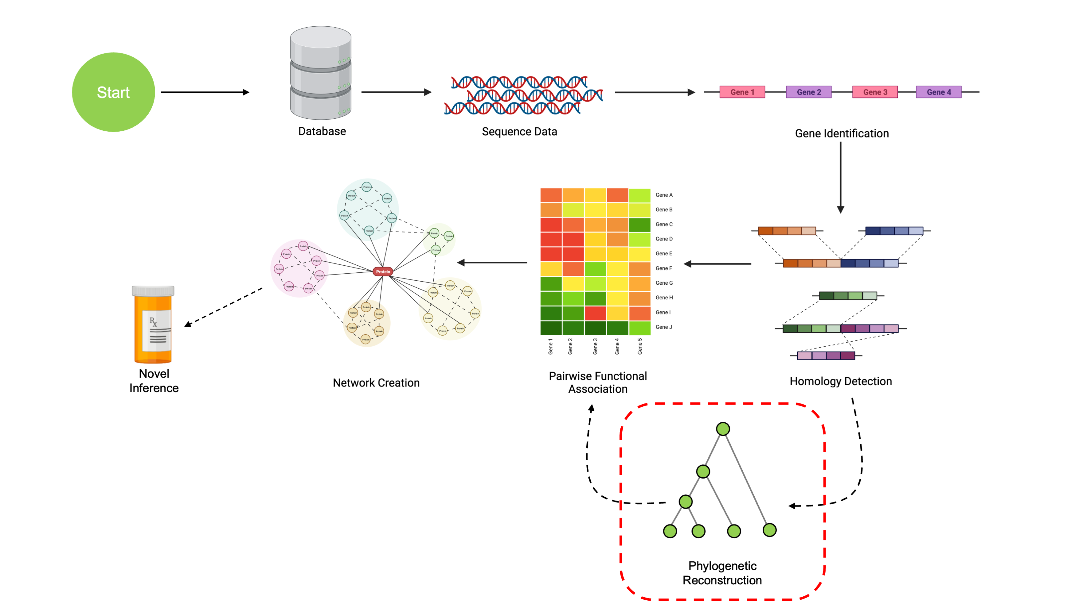
Phylogenetic Reconstruction
We’ve now learned how to find Clusters of Orthologous Genes (COGs)
from a set of sequences. The last thing we need for our final analysis
are phylogenetic reconstructions of each gene cluster. In this step,
we’ll build phylogenies for our COGs using the new
TreeLine() function introduced in the latest update of
DECIPHER. This analysis uses the third COG from the
previous section (if you don’t have it, you can download it below!).
library(DECIPHER)

# This is downloadable using the above button
# If you finished the previous page, this is MatchedSequences[[3]]
datafile <- '/path/to/testCOG.RData'
# Load in example COG
# Again, this is COG 3 from the previous section, which you can get with:
# testCOG <- MatchedSequences[[3]]

# If you don't have it, load it in this way
load(datafile, verbose=TRUE) # Should load 'testCOG'

# Let's make the names a little more concise
# These COGs exist in pairs with two lengths
# We'll code them as <Assembly><A/B>, where A is the longer sequence
# This renaming will make plotting look a little nicer
names(testCOG) <- c('1A', '1B', '2A', '2B',
                    '3B', '3A', '4B', '4A',
                    '5A', '5B')
testCOG <- testCOG[order(names(testCOG))]
# Let's look at the aligned COG sequences
testCOG
## DNAStringSet object of length 10:
## width seq names
## [1] 1215 GTGTACCTGTCCCACCTCACCGT...CGAGGGCGGCGCCGATGGCTGA 1A
## [2] 564 ATGGCTGAGACCCCCGCCCCGTT...GCCACGCGACACCTACGGCTGA 1B
## [3] 1215 GTGTACCTCTCCCACCTCACCGT...CGAGGGCGGCGCCGATGGCTGA 2A
## [4] 564 ATGGCTGAGACCCCCGCCCCGTT...GCCGCGCGACACCTACGGCTGA 2B
## [5] 1212 GTGCACCTGTCCCACCTGACCGT...CGGCGCCGGCGGGACCGAGGGT 3A
## [6] 565 ATGGCTGAGCAGCCCGCCTCGTT...CCCGCGCGACACCTACGGGTGA 3B
## [7] 1260 GTGCACCTGTCCCACCTCACCGT...GGACGGCGACGCCCGTGCGTGA 4A
## [8] 597 GTGCGTGAGCGCTCGCCGGAGCC...TCCGCGGGACACCTACGGCTGA 4B
## [9] 1215 GTGTACCTGTCCCACCTCACCGT...CGAGGGCGGCGCCGATGGCTGA 5A
## [10] 564 ATGGCTGAGACCCCCGCCCCGTT...GCCACGCGACACCTACGGCTGA 5B
# Since these are coding regions, AlignTranslation is preferred
testSeqs <- AlignTranslation(testCOG)

# Construct a gene tree from aligned sequences
treeCOG1 <- TreeLine(testSeqs, method='MP')

# Visualize the result
plot(treeCOG1, main='MP')
That’s all we need to construct a quick phylogenenetic tree in R! We
could also set the optional argument reconstruct=TRUE to
have TreeLine automatically reconstruct ancestral states at
each node.
However, TreeLine incorporates a wealth of functionality
past what is detailed here. In fact, this tree isn’t even the best tree
we can make! Let’s take a look at all the new features included in the
TreeLine() function.
Tree-Building Methods
Our first example used method='MP', meaning it
constructed a phyletic tree using a Maximum Parsimony method. However,
many more methods are available. TreeLine() implements
Maximum Parsimony (MP), Neighbor-Joining (NJ),
Ultrametric (complete, single,
UPGMA, WPGMA), and Maximum Likelihood
(ML) methods. Each of these have different strengths,
weaknesses, and assumptions. While an in-depth look at the difference
between these methods is outside the scope of this tutorial, I recently
published another
tutorial that goes into the mathematics of how these methods
work.
Example code for each of these:

# Neighbor-Joining
distMatrix <- DistanceMatrix(testSeqs)
treeNJ <- TreeLine(myDistMatrix=distMatrix, method='NJ')
plot(treeNJ, main='NJ')
# UPGMA tree
distMatrix <- DistanceMatrix(testSeqs)
treeUltra <- TreeLine(myDistMatrix=distMatrix, method='UPGMA')
plot(treeUltra, main='UPGMA')
Maximum-Likelihood trees are the most accurate, but also the slowest
to create. This method iteratively maximizes the likelihood of the tree
under a given sequence evolution model for a set of aligned sequences.
In the interest of time, this demo will set the maxTime
argument to prevent the algorithm from taking too long.
# Maximum Likehood
#   - Max runtime is set here to 30sec, default is as long as it takes
#   - maxTime expresses time in HOURS, not sec/min
#   - Note that method='ML' is the default setting
#   - Longer runtime will produce better results
treeML <- TreeLine(testSeqs, maxTime=(30/3600))
plot(treeML, main='Maximum-Likelihood')
Sequence Evolution Models
One question you’re probably asking is, “What is this ‘given sequence evolution model’?” That’s an excellent question!
By default, TreeLine() will test a variety of sequence
evolution models and pick the one that works best for your data. This
means that you shouldn’t typically have to worry about which model to
use.
However, what if we wanted to explicitly pick a certain model? What if we wanted to exclude a handful of models? Or what if we’re just curious what models are even being tested?
Fret not, for there is a solution. Models are passed to
TreeLine() as a list with two named entries,
$Nucleotide and $Protein. To look at the
default models tested, simply print out the MODELS variable
included from DECIPHER:
DECIPHER::MODELS## $Nucleotide
## [1] "JC69" "JC69+G4" "K80" "K80+G4" "F81" "F81+G4"
## [7] "HKY85" "HKY85+G4" "T92" "T92+G4" "TN93" "TN93+G4"
## [13] "SYM" "SYM+G4" "GTR" "GTR+G4"
##
## $Protein
## [1] "AB" "AB+G4" "BLOSUM62" "BLOSUM62+G4"
## [5] "cpREV" "cpREV+G4" "cpREV64" "cpREV64+G4"
## [9] "Dayhoff" "Dayhoff+G4" "DCMut-Dayhoff" "DCMut-Dayhoff+G4"
## [13] "DCMut-JTT" "DCMut-JTT+G4" "DEN" "DEN+G4"
## [17] "FLAVI" "FLAVI+G4" "FLU" "FLU+G4"
## [21] "gcpREV" "gcpREV+G4" "HIVb" "HIVb+G4"
## [25] "HIVw" "HIVw+G4" "JTT" "JTT+G4"
## [29] "LG" "LG+G4" "MtArt" "MtArt+G4"
## [33] "mtDeu" "mtDeu+G4" "mtInv" "mtInv+G4"
## [37] "mtMam" "mtMam+G4" "mtMet" "mtMet+G4"
## [41] "mtOrt" "mtOrt+G4" "mtREV" "mtREV+G4"
## [45] "mtVer" "mtVer+G4" "MtZoa" "MtZoa+G4"
## [49] "PMB" "PMB+G4" "Q.bird" "Q.bird+G4"
## [53] "Q.insect" "Q.insect+G4" "Q.LG" "Q.LG+G4"
## [57] "Q.mammal" "Q.mammal+G4" "Q.pfam" "Q.pfam+G4"
## [61] "Q.plant" "Q.plant+G4" "Q.yeast" "Q.yeast+G4"
## [65] "rtREV" "rtREV+G4" "stmtREV" "stmtREV+G4"
## [69] "VT" "VT+G4" "WAG" "WAG+G4"
## [73] "WAGstar" "WAGstar+G4"Nucleotide models include classic names like Jukes-Cantor
(JC69) and Felsenstein 1981 (F81), as well as
many others. The amino acid substitution models contain a mixture of
general models (e.g. BLOSUM62, Dayhoff), as
well as models tailored towards specific organisms
(e.g. Q.insect, HIVb).
To use a single model, simply create a list matching the structure of
MODELS, just with the models you want to include. To
exclude certain models, copy MODELS and remove the entries
you don’t want.
# Using a specific set of models
mySpecificModel <- list(Nucleotide=c('JC69', 'HKY85'))
specTree <- TreeLine(testSeqs, model=mySpecificModel, maxTime=(30/3600))
plot(specTree, main='Specific Set ML')
# Excluding Specific Models
myExcludedModel <- DECIPHER::MODELS
myExcludedModel$Protein <- NULL # Remove all protein models
myExcludedModel$Nucleotide <- myExcludedModel$Nucleotide[-1] # Remove JC69
exclTree <- TreeLine(testSeqs, model=myExcludedModel, maxTime=(30/3600))
plot(exclTree, main='Excluded Set ML')
Runtime Considerations
Runtime depends greatly on the tree construction method used. Phylogenetic reconstruction methods exhibit a tradeoff between accuracy and runtime; slower algorithms yield better performance.
Runtime scales with the number of genes and the length of each gene. For all below estimates, trials were done using a set of 100 genes with an aligned length of ~350 bases on a single core compute node with 1GB RAM. Reconstruction in amino acid space is slower on average than reconstruction in nucleotide space.
Maximum likelihood methods are the most accurate but also the slowest. For our test set of 100 genes, total runtime for nucleotide alignments takes on the order of 1-3 hours, and for amino acid alignments on the order of 10-12 hours.
Maximum parsimony methods are typically a good compromise between speed and accuracy. On our test set, total runtime was around 5-10 minutes for nucleotide alignments, and around 30 minutes for amino acid alignments.
All the other methods (Neighbor Joining, UPGMA, etc.) are extremely fast, but have much lower accuracy than MP/ML. Constructing a tree with these method (including building a distance matrix) takes less than 1 second.
Conclusion
That’s all we need to know how to do to generate phylogenies for our dataset. In order to conduct our final coevolutionary analysis, we’re going to need to build a gene tree for all of our COGs. I’ve precomputed these trees for us, so we can load those in in the next step without having to worry about long runtimes.
There are a few other parameters I didn’t mention in this writeup.
The most significant one for our use is reconstruct=TRUE,
as this reconstructs ancestral states (which will be important for later
analyses). There are also additional arguments for multiprocessing
(processors=1), using Laguerre quadrature for likelihoods
(quadrature=T/F), switching the type of information
criterion for ML trees
(informationCriterion=c('AICc', 'BIC')), and many others.
See the documentation page for more information on these–for now, we’ll
continue on to our final goal.