Gene Calling and Annotation with DECIPHER
Aidan Lakshman1
Source:vignettes/GeneCallingAnnotation.Rmd
GeneCallingAnnotation.Rmd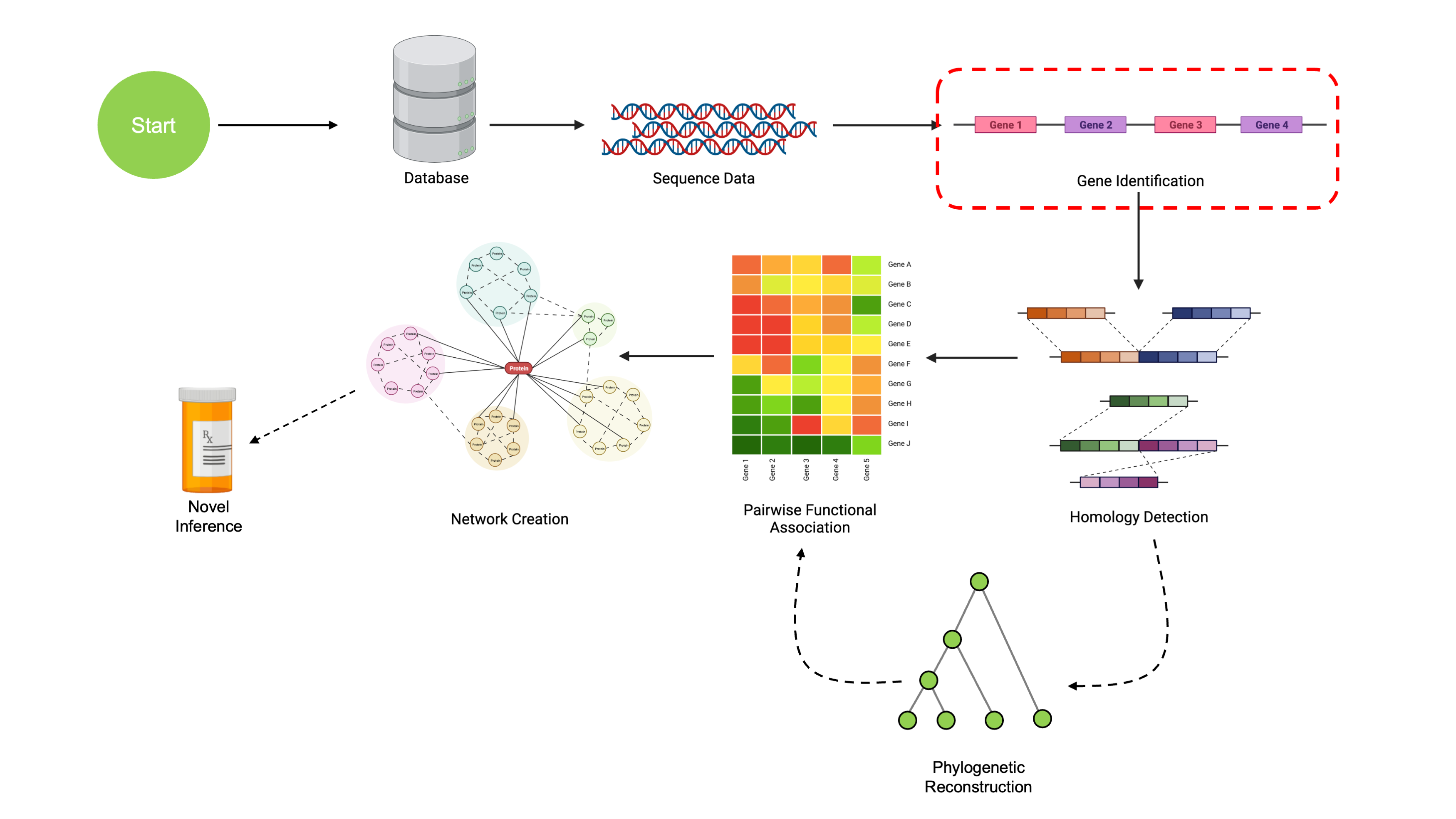
Gene Calling and Annotation
At this point, we’ve learned how to read in some genomic data, and have gained some basic familiarity working with it. The next step in our pipeline is to take a set of genomes, identify the coding regions in them, and predict the function of as many genetic regions as we can. We’ll start off by identifying the genes themselves.
Finding Genes
We’re going to keep using our Micrococcus dataset, but in
the interest of time we’ll focus on finding genes in a single sequence.
We’ll begin by reading in the data from a .fasta file, as
we did in the previous section.
library(DECIPHER)

# This file is downloadable at the above link
datafile <- '/path/to/SingleSeq.fa.gz'
dnaGenome <- readDNAStringSet(datafile)
aaGenome <- translate(dnaGenome)
Next, we’re going to identify the genes in our sequence using
FindGenes() from the DECIPHER package.
FindGenes() returns a Genes object with
information on where genes start and end in the genome.
geneLocs <- FindGenes(dnaGenome)
# `Genes` object
geneLocs
## Genes object of size 2,219 specifying:
## 2,219 protein coding genes from 75 to 4,653 nucleotides.
##
## Index Strand Begin End TotalScore ... Gene
## 1 1 0 256 1803 367.59 ... 1
## 2 1 0 2554 3669 255.97 ... 1
## 3 1 0 3691 4905 228.41 ... 1
## 4 1 0 4898 5461 74.94 ... 1
## 5 1 0 5819 7981 547.26 ... 1
## 6 1 0 8050 10746 686.36 ... 1
## ... with 2,213 more rows.We can then extract the sequences corresponding to each gene with
ExtractGenes().
genes <- ExtractGenes(geneLocs, dnaGenome, type='AAStringSet')
# Sequences corresponding to each gene
genes
## AAStringSet object of length 2219:
## width seq
## [1] 516 MVADQAVLSSWRSVVGSLEDDARVSARLMGFV...RKIRELMAERRTIYNQVTELTNEIKRKQRGA*
## [2] 372 MKFTVERDILTDAVSWAARSLSPRPPVPVLSG...SAPKPALLTGVNQEDGVVSDYRYLVMPVRIA*
## [3] 405 MYLSHLTVADFRSYRWADLELTPGSTVLLGAN...RQDAEGSEAVAAAAPVEGDIREPRREGGADG*
## [4] 188 MAETPAPFEPDRPDLALVQLRRVREAARERGE...TRIEVAGPQAPSWRKGPRTVRGGRGPRDTYG*
## [5] 721 MVDAMPENPAEEPTAASAAPNPEAVPDAVGQP...DAVFSMLMGEDVESRRTFIQQNAKDIRFLDV*
## ... ... ...
## [2215] 195 MSAENVTPAPEAEDAVVETPAGQGSRVAEQDD...KIVHDVVADAGLTSESEGEGARRHVVISADD*
## [2216] 333 MFEAILSPFRWLMSWLLGAFHSILEFAGLPAD...QAGRGGAVLNGEVVRQSGQRVQPQRKNRRRK*
## [2217] 123 MTVTPSPFVVLEPSREWGPLRALPSALLAGLL...PPGHRRWPPGRQPRILALNHPPIPPDLPQED*
## [2218] 133 MLPRDRRVRTPAEFRHLGRTGTRAGRRTVVVS...AEADYALLRRETVGALGKALKPHLPAASEHA*
## [2219] 46 MTKRTFQPNNRRRARKHGFRARMRTRAGRAILSARRGKNRAELSA*Of note is that FindGenes() assumes there are no introns
or frame shifts, and as a result performs best with prokaryotic
genomes.
Removing Non-Coding Regions
FindGenes() finds genes, but these may be coding or
non-coding genes. We’re more interested in the regions that are actually
translated into proteins, since these are what we’ll try to annotate
later. The FindNonCoding() function is developed
specifically for this purpose, to help distinguish between coding and
non-coding genes.
Using FindGenes() with FindNonCoding() in
this way also greatly improves the accuracy of FindGenes(),
since we won’t accidentally misidentify coding genes as non-coding
genes.
FindNonCoding() is used with three main datafiles
depending on the data to analyze:
-
data("NonCodingRNA_Archaea")for Archaeal data -
data("NonCodingRNA_Bacteria")for Bacterial data -
data("NonCodingRNA_Eukarya")for Eukaryotic data
These include pretrained models with common non-coding patterns for
the relevant domain of life. If these pretrained models are
insufficient, you can train your own dataset using
LearnNonCoding(), though this is outside the scope of this
workshop.
data("NonCodingRNA_Bacteria")
ncRNA <- NonCodingRNA_Bacteria

geneticRegions <- FindNonCoding(ncRNA, dnaGenome)

## Find annotations of noncoding regions
annotations <- attr(geneticRegions, "annotations")
geneMatches <- match(geneticRegions[,"Gene"], annotations)
noncodingAnnots <- sort(table(names(annotations)[geneMatches]))
# What noncoding regions have we found and annotated?
noncodingAnnots
##
## 5'_ureB-RF02514 Flavo_1-RF01705
## 1 1
## FMN_Riboswitch-RF00050 Glycine_Riboswitch-RF00504
## 1 1
## RNase_P_class_A-RF00010 SmallSRP-RF00169
## 1 1
## tmRNA-RF00023 tRNA-Asn
## 1 1
## tRNA-Asp tRNA-Cys
## 1 1
## tRNA-His tRNA-Phe
## 1 1
## tRNA-Trp tRNA-Tyr
## 1 1
## rRNA_16S-RF00177 rRNA_23S-RF02541
## 2 2
## rRNA_5S-RF00001 SAM_Riboswitch-RF00162
## 2 2
## TPP_Riboswitch-RF00059 tRNA-Gln
## 2 2
## tRNA-Lys tRNA-Met
## 2 2
## tRNA-Val tRNA-Glu
## 2 3
## tRNA-Ile tRNA-Pro
## 3 3
## tRNA-Thr tRNA-Ala
## 3 4
## tRNA-Arg tRNA-Gly
## 4 4
## tRNA-Ser tRNA-Leu
## 4 5FindNonCoding() returns a Genes object
identifying non-coding regions with annotations. We can pass this object
to FindGenes() to improve our identification of coding
regions, resulting in more accurate gene calling than just running
FindGenes() directly.
# Find Genes
genes <- FindGenes(dnaGenome, includeGenes=geneticRegions)
# Genes in the genome
genes
## Genes object of size 2,251 specifying:
## 2,193 protein coding genes from 99 to 4,653 nucleotides.
## 58 non-coding RNAs from 73 to 3,088 nucleotides.
##
## Index Strand Begin End TotalScore ... Gene
## 1 1 0 256 1803 376.48 ... 1
## 2 1 0 2554 3669 262.51 ... 1
## 3 1 0 3691 4905 225.34 ... 1
## 4 1 0 4898 5461 72.13 ... 1
## 5 1 0 5819 7981 558.05 ... 1
## 6 1 0 8050 10746 695.96 ... 1
## ... with 2,245 more rows.As before, we can pull out the sequences for these regions using
ExtractGenes(). Since these are all coding regions, we’ll
also translate them into amino acids.
# Find amino acid sequences corresponding to found genes
# May get a warning if we don't have an even multiple of 3 base pairs
geneSeqs <- ExtractGenes(genes, dnaGenome, type="DNAStringSet")
geneSeqs <- translate(geneSeqs)
geneSeqs## AAStringSet object of length 2251:
## width seq
## [1] 516 VVADQAVLSSWRSVVGSLEDDARVSARLMGFV...RKIRELMAERRTIYNQVTELTNEIKRKQRGA*
## [2] 372 VKFTVERDILTDAVSWAARSLSPRPPVPVLSG...SAPKPALLTGVNQEDGVVSDYRYLVMPVRIA*
## [3] 405 VYLSHLTVADFRSYRWADLELTPGSTVLLGAN...RQDAEGSEAVAAAAPVEGDIREPRREGGADG*
## [4] 188 MAETPAPFEPDRPDLALVQLRRVREAARERGE...TRIEVAGPQAPSWRKGPRTVRGGRGPRDTYG*
## [5] 721 VVDAMPENPAEEPTAASAAPNPEAVPDAVGQP...DAVFSMLMGEDVESRRTFIQQNAKDIRFLDV*
## ... ... ...
## [2247] 242 MTERGSAYERRPGLDPQDRGDRPAPVGQPAPP...KYGGAEPEILTVGEGLLPETTTVVRVSARPR*
## [2248] 195 MSAENVTPAPEAEDAVVETPAGQGSRVAEQDD...KIVHDVVADAGLTSESEGEGARRHVVISADD*
## [2249] 333 MFEAILSPFRWLMSWLLGAFHSILEFAGLPAD...QAGRGGAVLNGEVVRQSGQRVQPQRKNRRRK*
## [2250] 123 MTVTPSPFVVLEPSREWGPLRALPSALLAGLL...PPGHRRWPPGRQPRILALNHPPIPPDLPQED*
## [2251] 133 VLPRDRRVRTPAEFRHLGRTGTRAGRRTVVVS...AEADYALLRRETVGALGKALKPHLPAASEHA*Classification with IDTAXA
We now have a set of coding regions. Our last step for this section
is to try to annotate their function. This functionality is done with
IdTaxa() from the DECIPHER package.
IdTaxa() requires a training set, which can be obtained
in two ways. The first is to download them from DECIPHER’s downloads
page, which contains prebuilt training sets for a variety of
organisms. We’ll be using an Actinobacteria dataset obtained from this
website.
The other method is to build a training set yourself using
LearnTaxa(). This will not be covered in this workshop, but
more information is available on the DECIPHER documentation
for people that are interested.
In the interest of time, we’ll just classify the first 10 genes. Note
that our training set for IdTaxa() is trained on amino
acids, so we have to first call translate() on our DNA
sequences to be able to provide IdTaxa() with amino acid
sequences.
If this button doesn’t work, you can download it from the
DECIPHER
Downloads Page under “Training sets for functional classification
(amino acids)”. The correct training set for Microccocus is
KEGG Actinobacteria.
# RData training set file is downloadable from the above button.
# You can also download it directly from the DECIPHER website.

load('/path/to/KEGG_Actinobacteria_r95.RData')
# loads "trainingSet"
# Grab the first 10 genes extracted earlier
geneSeqSubset <- geneSeqs[1:10]

# Classify our sequences!
ids <- IdTaxa(geneSeqSubset, trainingSet)
Once we’ve finished calculating, we can either view the annotations directly, or plot them as a taxonomy.
# Looking at all results
ids
## A test set of class 'Taxa' with length 10
## confidence taxon
## [1] 100% Root; 09130 Environmental Information Processing; 09132 Signa...
## [2] 100% Root; 09120 Genetic Information Processing; 09124 Replication...
## [3] 100% Root; 09120 Genetic Information Processing; 09124 Replication...
## [4] 28% Root; unclassified_Root...
## [5] 96% Root; 09180 Brite Hierarchies; 09182 Protein families: geneti...
## [6] 100% Root; 09180 Brite Hierarchies; 09182 Protein families: geneti...
## [7] 36% Root; unclassified_Root...
## [8] 85% Root; unclassified_Root...
## [9] 27% Root; unclassified_Root...
## [10] 21% Root; unclassified_Root...
# Looking at a specific entry
ids[[1]]
## $taxon
## [1] "Root"
## [2] "09130 Environmental Information Processing"
## [3] "09132 Signal transduction"
## [4] "02020 Two-component system [PATH:ko02020]"
## [5] "K02313 dnaA, chromosomal replication initiator protein"
##
## $confidence
## [1] 100 100 100 100 100
# Plot the distribution of results
plot(ids, trainingSet)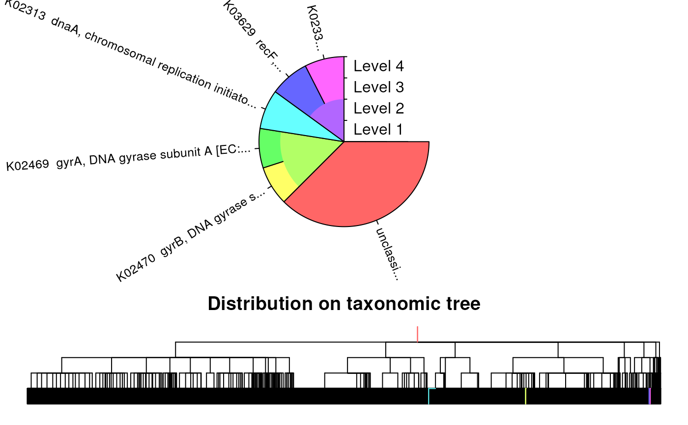
Runtime Considerations
Gene calling and annotation are both parallelizable; each compute node can process a single genome.
Runtime of gene calling depends on the length of each genome, but is
overall very fast. For a single Micrococcus genome (~2.5
megabase pairs), FindGenes takes approximately 40sec to
find ~2200 genes on a 2021 M1 MacBook Pro. The same operation on an
8.5Mbp Streptomyces genome takes around 5min to find ~7000
genes. FindNonCoding has a similar runtime,
Runtime of gene annotation depends on both the number of genes and the length of each gene (in base pairs). While compute could theoretically be parallelized to annotate one gene per compute node, this can be inefficient due to overhead incurred by copying the training set file to each node. Annotation on Streptomyces genes takes around 2 seconds per gene (ranging from 300-2000 bp).
Conclusion
We now have a way to identify genomic regions and annotate them with function. However, for comparative genomics we need some way to compare these genes across organisms so that we can draw conclusions at scale. In the next section, we’ll build on these techniques to find orthologous genomic regions.