Loading in Genome Data with DECIPHER
Aidan Lakshman1
Source:vignettes/LoadingGenomeData.Rmd
LoadingGenomeData.Rmd
Reading in Sequencing Data
In order to work with sequencing data, we first have to get it into R
in a format that allows us to work with it. The most commonly used
formats for genomic data are the XString and
XStringSet classes, which are available through the
Biostrings package.
XStrings come in four distinct flavors, depending on the
characters allowed:
-
DNAString, for DNA data (ATGC, plus gaps and ambiguity codes) -
RNAString, for RNA data (AUGC, plus gaps and ambiguity codes) -
AAString, for amino acid data (20 amino acids plusU,O, ambiguity codes, and unknown/gaps) -
BString, for any combination of any letters
When XString objects of the same type are combined, they
become an XStringSet. This provides an easy way to store
and work with genomics data. Below is an example of manually creating an
XStringSet:
library(DECIPHER) # Auto-imports Biostrings
# Making some toy sequences
sequences <- c('AGACTCGCA',
               'AGACGGTCA',
               'TCATTAGTT',
               'TGCACAAAA',
               'AGCTGTTGC')

sequenceSet <- DNAStringSet(sequences)
sequenceSet
## DNAStringSet object of length 5:
## width seq
## [1] 9 AGACTCGCA
## [2] 9 AGACGGTCA
## [3] 9 TCATTAGTT
## [4] 9 TGCACAAAA
## [5] 9 AGCTGTTGCWe can also translate DNA sequences to their amino acid counterparts
with translate().
translate(sequenceSet)## AAStringSet object of length 5:
## width seq
## [1] 3 RLA
## [2] 3 RRS
## [3] 3 SLV
## [4] 3 CTK
## [5] 3 SCCManually typing in sequences obviously isn’t a great system. Modern
sequencing data are typically in .fasta or
.fastq file format, so let’s look at a more realistic
use-case that reads in a data from a .fasta. We’re going to
be using an example from Micrococcus genomes obtained from NCBI
GenBank.
For purposes of the workshop, I’ve reduced the dataset to a single
Micrococcus gene. This expedites examples to allow for quick
processing. These sequences have been packaged into a single
.FASTA file (compressed into a .fa.gz file),
which you can download with the below button. Each gene is uniquely
identified with a three number code detailed on the Finding
COGs page.
# MicroFASTAtrimmed.fa.gz is loaded from the above button
# also available at extdata/LoadingData/ within this package

exampleSeqs <- '/path/to/MicroFASTAtrimmed.fa.gz'

exStringSet <- readDNAStringSet(exampleSeqs, format="fasta")
# we could also use format='fastq' for FASTQ datasets
exStringSet## DNAStringSet object of length 20:
## width seq names
## [1] 756 TCATCCTGCCAGCGCGGCGCGGG...CAATCGCTGAGGTGTTCGCCAT 13_8_653
## [2] 756 ATGGCGAACACCTCAGCGATTGA...CCGCGCCGCGCTGGCAGGATGA 18_1_1772
## [3] 756 TCATCCTGCCAGCGCGGCGCGGG...CAATCGCTGAGGTGTTCGCCAT 27_52_1555
## [4] 756 ATGGCGAACACCTCAGCGATTGA...CCGCGCCGCGCTGGCAGGATGA 29_16_724
## [5] 756 TCATCCTGCCAGCGCGGCGCGGG...CAATCGCTGAGGTGTTCGCCAT 30_15_973
## ... ... ...
## [16] 756 ATGGCGAACACCTCAGCGATTGA...CCGCGCCGCGCTGGCAGGATGA 78_1_1914
## [17] 756 TCATCCTGCCAGCGCGGCGCGGG...CAATCGCTGAGGTGTTCGCCAT 81_48_2187
## [18] 756 TCATCCTGCCAGCGCGGCGCGGG...CAATCGCTGAGGTGTTCGCCAT 82_2_146
## [19] 756 ATGGCGAACACCTCAGCGATTGA...CCGCGCCGCGCTGGCAGGATGA 90_1_931
## [20] 756 ATGGCGAACACCTCAGCGATTGA...CCGCGCCGCGCTGGCAGGATGA 91_1_936Success! Now we have a large example dataset to work with.
If we wanted to visualize these sequences, we can open them in a web
browser using BrowseSeqs() from DECIPHER:
BrowseSeqs(exStringSet)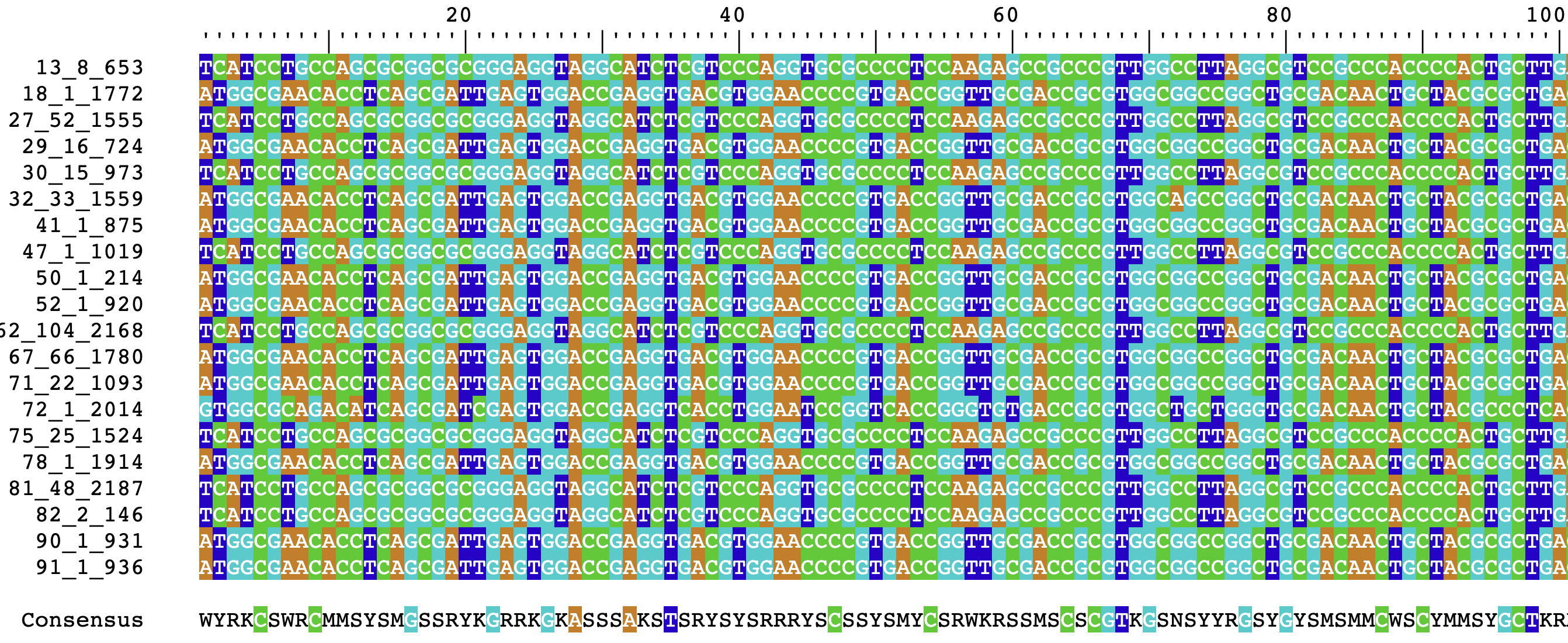
Aligning Sequences
Now that we have some sequences, let’s explore some of the ways we
can manipulate them. A complete demo of Biostrings is
outside the scope of this workshop, so we’ll just focus on functionality
added via DECIPHER.
A common analysis in bioinformatics is aligning sequences. This is
easily achievable with either the AlignSeqs() function or
the AlignTranslation() functions from
DECIPHER. AlignTranslation() aligns sequences
based on their translated amino acid sequences, and is significantly
more accurate for coding sequences (like the ones we’re working
with).
# Align the sequences
aliNoTranslate <- AlignSeqs(exStringSet, verbose=FALSE)

# Aligning using translated amino acid sequences
# These sequences are coding sequences, so this function will be more accurate
aliTranslate <- AlignTranslation(exStringSet, verbose=FALSE)

# Visualize through R
aliTranslate
## DNAStringSet object of length 20:
## width seq names
## [1] 951 -----------------------...CAATCGCTGAGGTGTTCGCCAT 13_8_653
## [2] 951 ATGGCGAACACCTCAGCGATTGA...---------------------- 18_1_1772
## [3] 951 -----------------------...CAATCGCTGAGGTGTTCGCCAT 27_52_1555
## [4] 951 ATGGCGAACACCTCAGCGATTGA...---------------------- 29_16_724
## [5] 951 -----------------------...CAATCGCTGAGGTGTTCGCCAT 30_15_973
## ... ... ...
## [16] 951 ATGGCGAACACCTCAGCGATTGA...---------------------- 78_1_1914
## [17] 951 -----------------------...CAATCGCTGAGGTGTTCGCCAT 81_48_2187
## [18] 951 -----------------------...CAATCGCTGAGGTGTTCGCCAT 82_2_146
## [19] 951 ATGGCGAACACCTCAGCGATTGA...---------------------- 90_1_931
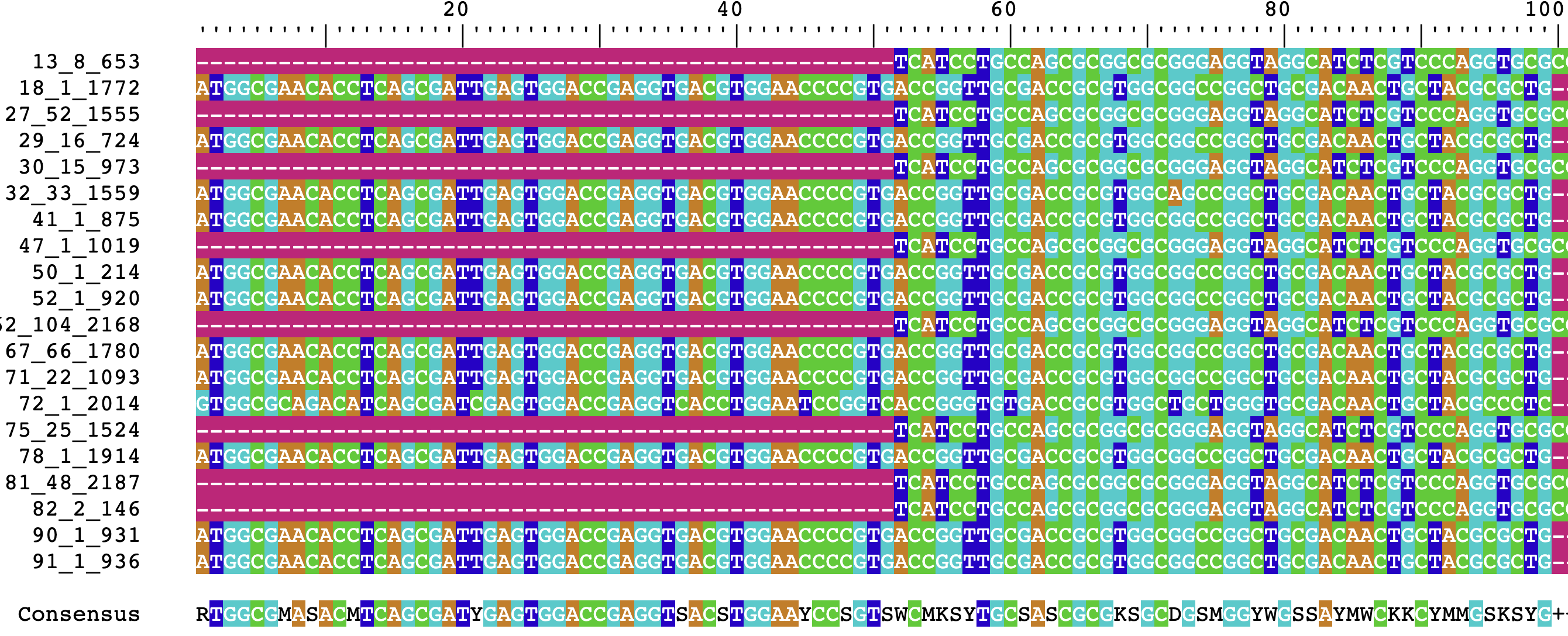
## [20] 951 ATGGCGAACACCTCAGCGATTGA...---------------------- 91_1_936Alignments tend to start with a lot of gaps, and as a result viewing
them through R isn’t always super informative. As before, we can
visualize this alignment in a much better way using
BrowseSeqs():
BrowseSeqs(aliTranslate)The output should resemble the following:
Big Data with DECIPHER
One of DECIPHER’s unique features is the ability to work
with massive amounts of data. DECIPHER incorporates a rich
API for working with sequencing data stored in SQLite files. These allow
users to work with enormous amounts of data (ex. hundreds of thousands
of sequences) while providing the following benefits:
- Space optimization
- Fast random access
- Concurrent use from multiple queries/users
- Reliable and cross-platform storage
For more information on all the benefits of using databases with
DECIPHER, check out the DECIPHER
publication.
Setting up a DECIPHER database takes a few extra lines
of code, but it’s worth it! Let’s start by creating a connection to a
SQLite database.
# You can set this to any path, use a non-tempfile for long term storage
DBPATH <- tempfile()
dbConn <- dbConnect(SQLite(), DBPATH)
Now we have a connection to a database! I used
tempfile() for a temporary file, but you could have also
added a filepath to a non-temporary file. Note that if the file does not
exist, it will be automatically created.
Now it’s time to start populating our database with sequences! This
is done with Seqs2DB() with the following syntax:
# All sequences must be identified with a unique quantifier
# This has to be a character vector; we can make it 1:length(exStringSet)
identifiers = as.character(seq_along(exStringSet))
Seqs2DB(seqs=exStringSet, type='XStringSet',
        dbFile=dbConn, identifier=identifiers)
## Adding 20 sequences to the database.
##
## 20 total sequences in table Seqs.
## Time difference of 0.06 secsWe can also write sequences directly from a FASTA file
to our database. In this code, we’re using replaceTbl=TRUE
so that we replace our table with the sequences (rather than add the
same set twice).
# We can also directly import from a FASTA file
# FASTA files
Seqs2DB(seqs=exampleSeqs, type='FASTA',
        dbFile=dbConn, identifier=identifiers,
        replaceTbl=TRUE)
##
Reading FASTA file chunk 1
##
## 20 total sequences in table Seqs.
## Time difference of 0.03 secsNow that we have our database, what do we do with it?
To start, we can run BrowseDB(), a function analogous to
BrowseSeqs() but for DECIPHER databases.
Instead of showing sequences, this visualization shows entries in the
database that can be queried.
BrowseDB(dbConn)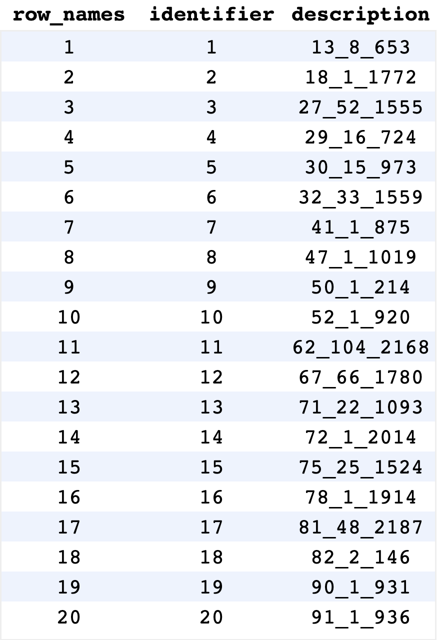
If we want to read the sequences back into R as an
XStringSet, we use SearchDB().
dbStringSet <- SearchDB(dbConn)## Search Expression:
## select row_names, sequence from _Seqs where row_names in (select row_names
## from Seqs)
##
## DNAStringSet of length: 20
## Time difference of 0 secs
dbStringSet## DNAStringSet object of length 20:
## width seq names
## [1] 756 TCATCCTGCCAGCGCGGCGCGGG...CAATCGCTGAGGTGTTCGCCAT 1
## [2] 756 ATGGCGAACACCTCAGCGATTGA...CCGCGCCGCGCTGGCAGGATGA 2
## [3] 756 TCATCCTGCCAGCGCGGCGCGGG...CAATCGCTGAGGTGTTCGCCAT 3
## [4] 756 ATGGCGAACACCTCAGCGATTGA...CCGCGCCGCGCTGGCAGGATGA 4
## [5] 756 TCATCCTGCCAGCGCGGCGCGGG...CAATCGCTGAGGTGTTCGCCAT 5
## ... ... ...
## [16] 756 ATGGCGAACACCTCAGCGATTGA...CCGCGCCGCGCTGGCAGGATGA 16
## [17] 756 TCATCCTGCCAGCGCGGCGCGGG...CAATCGCTGAGGTGTTCGCCAT 17
## [18] 756 TCATCCTGCCAGCGCGGCGCGGG...CAATCGCTGAGGTGTTCGCCAT 18
## [19] 756 ATGGCGAACACCTCAGCGATTGA...CCGCGCCGCGCTGGCAGGATGA 19
## [20] 756 ATGGCGAACACCTCAGCGATTGA...CCGCGCCGCGCTGGCAGGATGA 20SearchDB() incorporates far more options than just
returning all the sequences in the database. If we had a database of a
million sequences, we would likely crash our R environment trying to
load them all in. Instead, we can use the following options:
# Limit amount returned to first 10
SearchDB(dbConn, limit=10)

# Look for a specific identifier
# BrowseDB() is useful here for determining what the identifiers are
SearchDB(dbConn, identifier = 'example identifier')

# Run SQL queries
#     This clause is appended to the end of a `WHERE ... ` call
SearchDB(dbConn, clause = 'identifier in ("1", "2", "3")')
Once we’re done working with the database, it’s important to
disconnect any open SQLite connections.
dbDisconnect(dbConn)Many DECIPHER functions use databases rather than
XStringSet objects for speed and efficiency. As an example,
let’s look at the FindSynteny() function.
FindSynteny() allows us to look at syntenic hits between
sequences without aligning them. The result allows us to easily
visualize differences between two sequences without the computational
cost of sequence alignment. Let’s look at an example of finding syntenic
hits between the first 6 sequences in our set.
to_select <- c(1,3,5,8)
synData <- exStringSet[to_select]

names(synData) <- as.character(to_select)

# Initialize our database
DBPATH <- tempfile()
dbConn <- dbConnect(SQLite(), DBPATH)
Seqs2DB(synData, "XStringSet", dbConn, identifier=as.character(to_select))

syn <- FindSynteny(dbConn)
dbDisconnect(dbConn)

pairs(syn)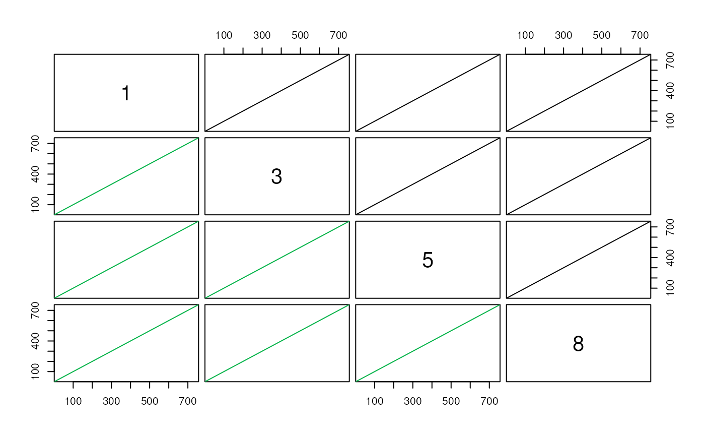
What are we looking at with this plot? Each plot compares two genomes, and each point is a syntenic hit between the two genomes. The X position of the point is its location on the first genome, and the Y position is its position on the second genome. If we had identical genomes, we would expect to see a diagonal line \(y=x\), indicating that all bases occur at the same place in both genomes. Gaps indicate areas that do not match, and points off the diagonal indicate matching areas in different places on each genomes. These particular examples are highly syntenic, so they all resemble the line \(y=x\).
We’ll see a more in-depth example of using Synteny
objects returned by FindSynteny() later on.
Runtime Considerations
Loading genomes is fairly fast; each sequence takes on the order of 1-2 seconds. The runtime of these operations are rarely significant in the overall runtime of the entire pipeline.
When implementing at scale on a compute cluster, it may be more efficient to use NCBI’s Entrez Search to download genomes on the fly; this adds some runtime overhead but improves memory efficiency on individual compute nodes.