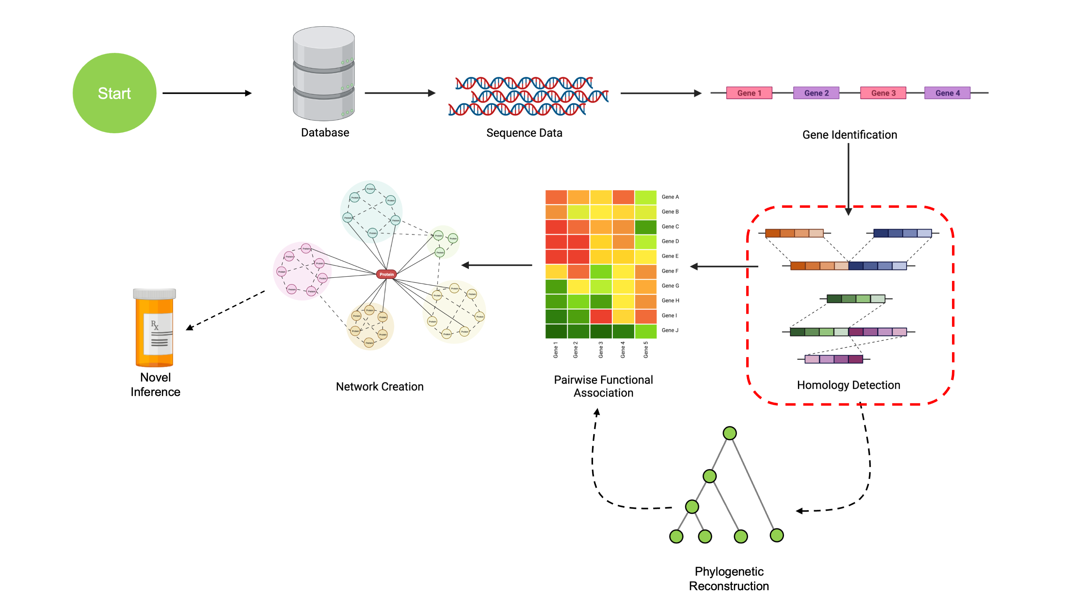
Finding COGs
We’ve now learned some ways to load genomic data into R, as well as ways to find and annotate genomic sequences. Once we have annotated sequence data, we’ll want to find genes that are orthologous. Orthologous genes are genes that derive from some common ancestral gene in the past. This is how we can “match” up genes from different organisms. It isn’t guaranteed that these genes have preserved function since diverging from their ancestral state, but it does give us insight into the evolution of genes over time. Sets of orthologous genes will referred to as COGs (Clusters of Orthologous Genes).
Building Our Dataset
We’re going to continue using our Micrococcus genomes from NCBI, this time on a subset of 5 genomes. As mentioned in previous sections, the complete data are available here, and you are more than welcome to try these analyses out with more genomes at any time!
All the code in this section will work on larger datasets, you may just have to wait a little while. See the Conclusions page for more information on running these analyses at scale.
For this analysis, we’re downloading the genomic data as
.fasta files along with precalculated annotations as
.gff files. We could have also called genes and annotated
them in DECIPHER using the method in the previous page,
this just provides an example of using prebuilt annotations for a more
thorough overview of different use cases.
# Using DECIPHER's database API!
DBPATH <- tempfile()
# Pull out just the folders we want
genomedirs <- list.files(COGExampleDir, full.names = TRUE)
genomedirs <- genomedirs[grep('json', genomedirs, fixed=T, invert=T)]
# Initializing our GeneCalls list
GeneCalls <- vector('list', length=length(genomedirs))
for (i in seq_along(genomedirs)){
subfiles <- list.files(genomedirs[i], full.names = TRUE)
# Find the FASTA file and the GFF annotations file
fna_file <- subfiles[which(grepl('.*fna$', subfiles))]
gff_file <- subfiles[which(grepl('.*gff$', subfiles))]
# Read in sequence to database
Seqs2DB(seqs = fna_file,
type = "FASTA",
dbFile = DBPATH,
identifier = as.character(i), # Sequences must be identified by number
verbose = TRUE)
# Read in annotations
GeneCalls[[i]] <- gffToDataFrame(GFF = gff_file,
Verbose = TRUE)
}
names(GeneCalls) <- seq_along(GeneCalls) # Must have number IDs here too
# Note again that we could have used `FindNonCoding` and `FindGenes`
# Rather than rely on having precomputed GeneCalls from a .gffFinding Orthologous Pairs
Now we have all of our data read in successfully. Next, we’ll have to
find pairs of orthologous genes. This is accomplished by means of the
NucleotideOverlap() and PairSummaries()
functions from SynExtend. NucleotideOverlap()
uses a Synteny object and determines where genomic features
are connected by syntenic hits. PairSummaries determines
pairs of genes that are orthologous by parsing these connected
regions.
Note: Several methods here are commented out. This is to
save time within the workshop, since we have a lot to cover in a
relatively short time. Running the output of
PairSummaries() through BlockExpansion() and
BlockReconciliation() improves accuracy of our final
identified orthologous regions at the cost of runtime. I encourage
readers to try out this functionality on their own in the absence of
tight time constraints.
Syn <- FindSynteny(dbFile = DBPATH,
verbose = TRUE)
Overlaps <- NucleotideOverlap(SyntenyObject = Syn,
GeneCalls = GeneCalls,
Verbose = TRUE)
Pairs <- PairSummaries(SyntenyLinks = Overlaps,
GeneCalls = GeneCalls,
DBPATH = DBPATH,
PIDs = FALSE, # Set to TRUE for better accuracy (slower)
Score = FALSE, # Set to TRUE for better accuracy (slower)
Verbose = TRUE)
# These methods only work if we set PIDs and Score to TRUE
# Unfortunately we don't have time in this workshop to use these
# Feel free to try them out on your own with a larger dataset!
# P02 <- BlockExpansion(Pairs = P01,
# DBPATH = DBPATH,
# Verbose = TRUE,
# NewPairsOnly = FALSE)
# P03 <- BlockReconciliation(Pairs = P02,
# PIDThreshold = 0.75,
# SCOREThreshold = 200,
# Verbose = TRUE)
# Pairs <- P03[P03$PID > 0.4, ]
head(Pairs)## p1 p2 ExactMatch Consensus TotalKmers MaxKmer p1FeatureLength
## 1 1_1_1 2_1_1997 1429 0.99901827 14 391 1548
## 2 1_1_2 2_1_1998 1069 1.00000000 7 302 1116
## 3 1_1_3 2_1_1999 1012 1.00000000 15 176 1215
## 4 1_1_4 2_1_1999 8 0.01038438 1 8 564
## 5 1_1_4 2_1_2000 477 1.00000000 4 342 564
## 6 1_1_5 2_1_1044 274 0.96977256 12 39 2151
## p2FeatureLength Adjacent TetDist PIDType PredictedPID
## 1 1554 1 0.008090447 AA 0.98178450
## 2 1116 2 0.000000000 AA 0.98793709
## 3 1215 1 0.007651500 AA 0.94297930
## 4 1215 0 0.052066912 AA 0.06709154
## 5 564 1 0.005041760 AA 0.98409819
## 6 2106 0 0.026607476 AA 0.53031474Finding COGs
From these pairwise orthologous regions, we can finally determine
COGs using the DisjointSet() function from
SynExtend. This function analyzes pairs to determine which
orthologs are (dis)connected. Future work will look into smarter ways to
determine COGs from pairwise orthologies, but method currently shows
strong performance.
COGSets <- DisjointSet(Pairs = Pairs,
Verbose = TRUE)
COGSets[1:3]## $`1`
## [1] "1_1_1" "2_1_1997" "3_1_422" "4_1_375" "5_1_1"
##
## $`2`
## [1] "1_1_2" "2_1_1998" "3_1_421" "4_1_374" "5_1_2"
##
## $`3`
## [1] "1_1_3" "1_1_4" "2_1_1999" "2_1_2000" "3_1_419" "3_1_420"
## [7] "4_1_372" "4_1_373" "5_1_3" "5_1_4"This object is a list of character vectors, where each element of each character vector uniquely identifies a gene. The annotation schema is the following:
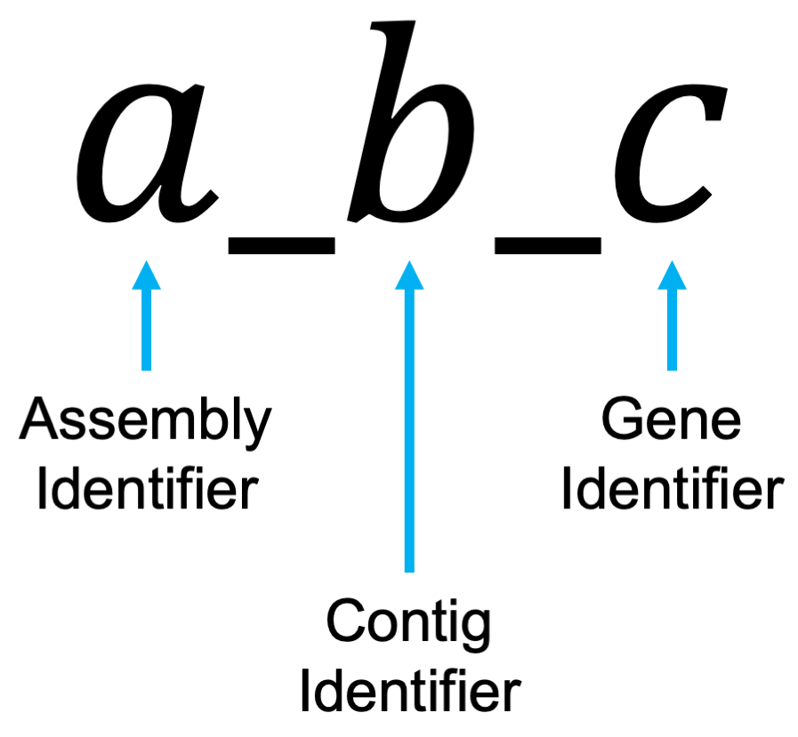
Assembly refers to the assembly (1-5 for this data), strand refers to
which chromosome the gene is found on, and the gene identifier is a
unique number for each gene. For example, 2_1_1999 refers
to the 1999th gene from the 2nd assembly (genome)
on the 1st chromosome.
Once we have these COGs, we can use ExtractBy to pull
out the sequences corresponding to each genomic region in each COG.
# Extract sequences for COGs with at least 5 orthologs
Sequences <- ExtractBy(x = Pairs,
y = DBPATH,
z = COGSets[lengths(COGSets) >= 5],
Verbose = TRUE)
# These come back in different orders, so let's match them up
allnames <- lapply(Sequences, names)
COGMapping <- sapply(COGSets, \(x){
which(sapply(allnames, \(y) setequal(x,y)))
}
)
COGMapping <- COGMapping[sapply(COGMapping, \(x) length(x) > 0)]
MatchedCOGSets <- COGSets[names(COGMapping)]
MatchedSequences <- Sequences[unlist(COGMapping)]
names(MatchedSequences) <- names(COGMapping)
MatchedCOGSets[1:3]## $`1`
## [1] "1_1_1" "2_1_1997" "3_1_422" "4_1_375" "5_1_1"
##
## $`2`
## [1] "1_1_2" "2_1_1998" "3_1_421" "4_1_374" "5_1_2"
##
## $`3`
## [1] "1_1_3" "1_1_4" "2_1_1999" "2_1_2000" "3_1_419" "3_1_420"
## [7] "4_1_372" "4_1_373" "5_1_3" "5_1_4"
MatchedSequences[1:3]## $`1`
## DNAStringSet object of length 5:
## width seq names
## [1] 1548 GTGGTGGCAGACCAGGCCGTGCT...AGCGGAAGCAGCGCGGCGCCTGA 1_1_1
## [2] 1554 GTGGTGGCAGACCAGGCCGTGCT...AGCGGAAACAGCGCGGCGCCTGA 2_1_1997
## [3] 1551 GTGGTGGCAGACCAGGCCGTGCT...AGCGCAAGCAGCGCGGCGCCTGA 3_1_422
## [4] 1536 ATGGCGGCGGACCAGGAGCTGCT...AGCGCAAGCAGCGCGGGGCCTGA 4_1_375
## [5] 1548 GTGGTGGCAGACCAGGCCGTGCT...AGCGGAAGCAGCGCGGCGCCTGA 5_1_1
##
## $`2`
## DNAStringSet object of length 5:
## width seq names
## [1] 1116 GTGAAGTTCACCGTCGAACGCGA...TGATGCCGGTGCGCATCGCCTGA 1_1_2
## [2] 1116 GTGAAGTTCACCGTCGAACGCGA...TGATGCCGGTGCGCATCGCCTGA 2_1_1998
## [3] 1115 GTGAAGTTCACCGTCGAACGCGA...TGATGCCGGTGCGCATCGCCTGA 3_1_421
## [4] 1116 GTGAAGTTCACCGTGGCACGCGA...TGATGCCCGTCCGCCTGACCTGA 4_1_374
## [5] 1116 GTGAAGTTCACCGTCGAACGCGA...TGATGCCGGTGCGCATCGCCTGA 5_1_2
##
## $`3`
## DNAStringSet object of length 10:
## width seq names
## [1] 1215 GTGTACCTGTCCCACCTCACCGT...CGAGGGCGGCGCCGATGGCTGA 1_1_3
## [2] 564 ATGGCTGAGACCCCCGCCCCGTT...GCCACGCGACACCTACGGCTGA 1_1_4
## [3] 1215 GTGTACCTCTCCCACCTCACCGT...CGAGGGCGGCGCCGATGGCTGA 2_1_1999
## [4] 564 ATGGCTGAGACCCCCGCCCCGTT...GCCGCGCGACACCTACGGCTGA 2_1_2000
## [5] 565 ATGGCTGAGCAGCCCGCCTCGTT...CCCGCGCGACACCTACGGGTGA 3_1_419
## [6] 1212 GTGCACCTGTCCCACCTGACCGT...CGGCGCCGGCGGGACCGAGGGT 3_1_420
## [7] 597 GTGCGTGAGCGCTCGCCGGAGCC...TCCGCGGGACACCTACGGCTGA 4_1_372
## [8] 1260 GTGCACCTGTCCCACCTCACCGT...GGACGGCGACGCCCGTGCGTGA 4_1_373
## [9] 1215 GTGTACCTGTCCCACCTCACCGT...CGAGGGCGGCGCCGATGGCTGA 5_1_3
## [10] 564 ATGGCTGAGACCCCCGCCCCGTT...GCCACGCGACACCTACGGCTGA 5_1_4Runtime Considerations
Finding COGs is comprised of multiple steps that are almost all parallelizable.
Each pair of genomes can be compared on a separate compute node. If
BlockExpansion and BlockReconciliation are
used, total runtime is on the order of 5-20 minutes per pair. Runtime
scales with the number of gene calls and the length of each gene.
Skipping BlockExpansion and
BlockReconciliation can improve runtime by a factor of
2-5x, but decreases accuracy.
Reconciling pairwise orthology into COGs using
DisjointSets does not parallelize well, but is a fast
operation overall. Runtime scales on the number of pairwise orthology
predictions. Reconciling pairwise orthology predictions from 2.2 million
Streptomyces gene calls takes on the order of 20 minutes
total.
Conclusion
Now we know how to generate COGs from a dataset of genomes and gene calls. We could have also generated gene calls ourselves, but if high quality gene annotations are already available (e.g. on NCBI), it makes sense to use them. Remember that this example is intentionally small so it can fit into our workshop within the time constraints–I highly encourage experimenting with other, larger datasets!